
SIMULATION MODELLING OF IRON ORE PRODUCTION
SYSTEM AND QUALITY MANAGEMENT
J. E. Everett
Faculty of Economics and Commerce, University of Western Australia, Nedlands, Western Australia
Keywords: Decision Support Systems, Simulation, Operational logistics, Modelling methodologies.
Abstract: Iron ore is railed several hundred kilometres from open-cut mines inland, to port facilities, then processed to
lump and fines products, blended and the lump product re-screened ready for shipment, mainly to Asia.
Customers use the ore as principal feed in steel production. Increasing demand and price, especially from
China, requires expansion of existing mines and planning of new operations. Expansion planning of the
operational logistics, maintaining acceptable product quality, has been greatly helped by simulation
modelling described in this paper.
1 INTRODUCTION
Ore from open-cut mines in the Pilbara region of
Western Australia is railed a few hundred kilometres
to a port where the ore is processed and blended for
shipment, mainly to Asia. Customers use the ore as
feed in steel production. Figure 1 shows a simplified
ore flow, although many operational variations exist.
Increased iron ore demand has required a review
of capacity. To increase tonnage safely, at minimum
cost and acceptable quality, processes need to be
upgraded, existing mines and infrastructure
expanded, and new mines brought on line.
Assessment requires informed choices between
operation and infrastructure development options
that differ in capital and operating costs. Many
alternatives exist for mining, ore processing,
stockpiling, railing and ship loading operations.
Expansion options must be assessed for their
effect on product quality. Customers assess quality
by cargo grade, and inter-cargo grade variability. As
well as iron, several impurities, principally
phosphorus, silica, and alumina are important.
Simulation models of expansion options enable
mining and handling alternatives to be compared.
They consider tonnage capabilities and the variation
in product quality, a vector of iron, phosphorus,
silica, and alumina grades. These grades shows
complex serial and cross correlations, so synthetic
data cannot readily be constructed. Production was
simulated from historic data of geologically similar
ore, statistically adjusted to match potential
operations.
The models were written in Excel™, with Visual
Basic (VBA) macros, making full use of the
graphical capabilities. Simulations described here
have been used to evaluate expansion and
development options. The results have helped assess
the effect on product quality for many processing
and equipment options for capacity expansion.
2 THE PRODUCTION SYSTEM
The Pilbara produces about 200 million tones of iron
ore per year, sold as two product types; lump (6 to
31mm) and fines (under 6mm). Increased demand
for iron ore, mainly by China, requires producers to
increase tonnage, by upgrading existing mines and
opening new mines. Assessment requires informed
choices between alternative modes of operation and
development, which differ greatly in expected
capital and operating costs. Reviewing the many
options that exist is complex, and greatly aided by
simulation. This paper describes simulations carried
out to assess product grade quality for potential
expansion developments. Simulations were based on
proposed infrastructure and capacity options
identified from engineering studies. They were set
up so the impact of changes to operating practices on
product grade quality could also be assessed.
300
E. Everett J. (2006).
SIMULATION MODELLING OF IRON ORE PRODUCTION SYSTEM AND QUALITY MANAGEMENT.
In Proceedings of the Eighth International Conference on Enterprise Information Systems - AIDSS, pages 300-303
DOI: 10.5220/0002443203000303
Copyright
c
SciTePress

2.1 Production Flow
At the mine, monthly mine plans are designed for
cost efficient use of the resource. Ore blocks are
blasted and assigned into floor stocks of consistent
geology and composition using analysis from
samples taken during the drilling of the blast holes.
Each day, ore to mine is selected from floor stocks,
based on target grade, current deviation from target,
and cost efficient mine development. In our
example, ore from four mines goes 400 kilometres to
the port to be crushed, screened into lump and fines
products and blended by stacking onto 150 kilotonne
stockpiles. Ore from completed stockpiles is
reclaimed, loaded onto ships, and transported to
customers. Everett (1996, 2001) discusses iron ore
quality control. Kamperman et al (2002) describe
application of the methods to a Pilbara operation.
2.2 The Cost of Quality
The objective is to deliver the required ore tonnage,
at minimum total cost and of quality acceptable to
the customer. Quality is based on iron content and
the percentage of impurities such as phosphorus,
silica and alumina. There are two key criteria: cargo
grade and inter-cargo variability. Customers require
each shipment to be close to target composition.
Agreed tolerances are used to guide decisions,
throughout the production process. Excessive inter-
cargo variation potentially affects price and sales
tonnages. This cost, containing an element of risk, is
hard to evaluate quantitatively. Blending and re-
handling to improve uniformity adds to operating
cost, a potential trade off against quality.
3 SIMULATION METHODS
Expansion options were developed, for alternative
production and handling concepts from mine to ship
loading. Their quality implications were evaluated
by simulation. Long-term grade variability (> one
month) is controlled by the mine plan. Short-term
inter-cargo variability is controlled by the
operational process, and is the assessment metric.
3.1 Data Preparation
Production data show complex serial and cross
correlation (for iron, silica, alumina and phosphorus)
that is ascribed to the orderly mining of blast blocks
and the daily decisions to control grade.
Historic data were used to generate the required
input data for modelling future mining production in
the simulations, so that the existing serial and cross
correlations were maintained. However, historic data
contained long-term variation that could mask any
incremental improvements identified in the
simulations; planned new mines lacked historic data,
and had expected means grades differing from
existing mines.
Synthetic data for new mines were created from
existing mines of similar geology. Long-term trends
were filtered out using Fourier analysis. Means and
standard deviations were then adjusted to create
synthetic data matching planned production. The
data preparation model allowed the standard
deviation to be reduced, simulating increased effort
within the mine to control short-term variability,
through such activities as selective mining and pre-
crusher stockpiling.
Figure 1: A Typical Iron Ore Production System.
SIMULATION MODELLING OF IRON ORE PRODUCTION SYSTEM AND QUALITY MANAGEMENT
301

4 SIMULATION MODELS
Dedicated simulation packages need specialists to
run and interpret the results, usually with cost and
licensing restrictions. They represent a barrier to
practitioners who must learn a new package if they
are to run the models independently.
Developing the system in Excel
TM
allowed
mining engineers and operators to explore
alternative policies and scenarios, using domain
knowledge unavailable to the designer of the
simulation model. Graphing and analysing of results
was built in, so minimal ongoing assistance was
required from the simulation provider.
Constructing a simulation model in a spreadsheet
workbook, run by VBA macros, is as easy as in a
dedicated simulation package. The spreadsheet’s
data input and output reporting and graphing
capabilities are fuller than are generally found in a
simulation package. The industry user, familiar with
spreadsheets and their potential, can suggest
improvements to the simulation model. The VBA
macro coding is hidden from the practitioner, who
can use it by means of inbuilt buttons and menus.
The simulation model comprised three VBA
macros: reading in parameters to set up the
simulation; running the simulation the required
number of time periods, and finally using Excel’s
statistical and graphing power to report the results.
The models were used to study the effects of
controllable variables (such as stockpile sizes and
stockpiling methods) and uncontrollable variables
(such as cargo sizes). The worksheets specified
parameters and policy choices, displayed simulation
progress, and reported and graphed a performance
summary for any simulation run. For reproducible
results, a year or more of production had to be
simulated.
The simulation was time-sliced (at six hour
intervals) rather than event-driven. In each time
interval, ore is mined and trains loaded, while at the
port trains arrive and are unloaded, crushed and
stacked to stockpiles, ships can arrive, commence
being loaded from an available stockpile (or wait if
none are available) continue being loaded, and
depart when full. Simulations were run to explore
the effect of steadily changing the values of a
particular parameter, or a set of parameters.
Separate workbook models were written to
simulate the Mine and Port operations. They could
be run individually, or be run together by a Master
model, for a sequence of scenarios. Space limitation
limits discussion here to the Port model.
5 PORT MODEL EXAMPLE
The Port model has six worksheets, simulating stack
and reclaim of ore from train to ship.
The “Input Rakes” sheet imports a set of 2,048
train rakes from the “Output” sheet of the Mine
model file. Incoming trains are from either of two
pits that have systematically different mean grade, to
reflect planned trends in mining.
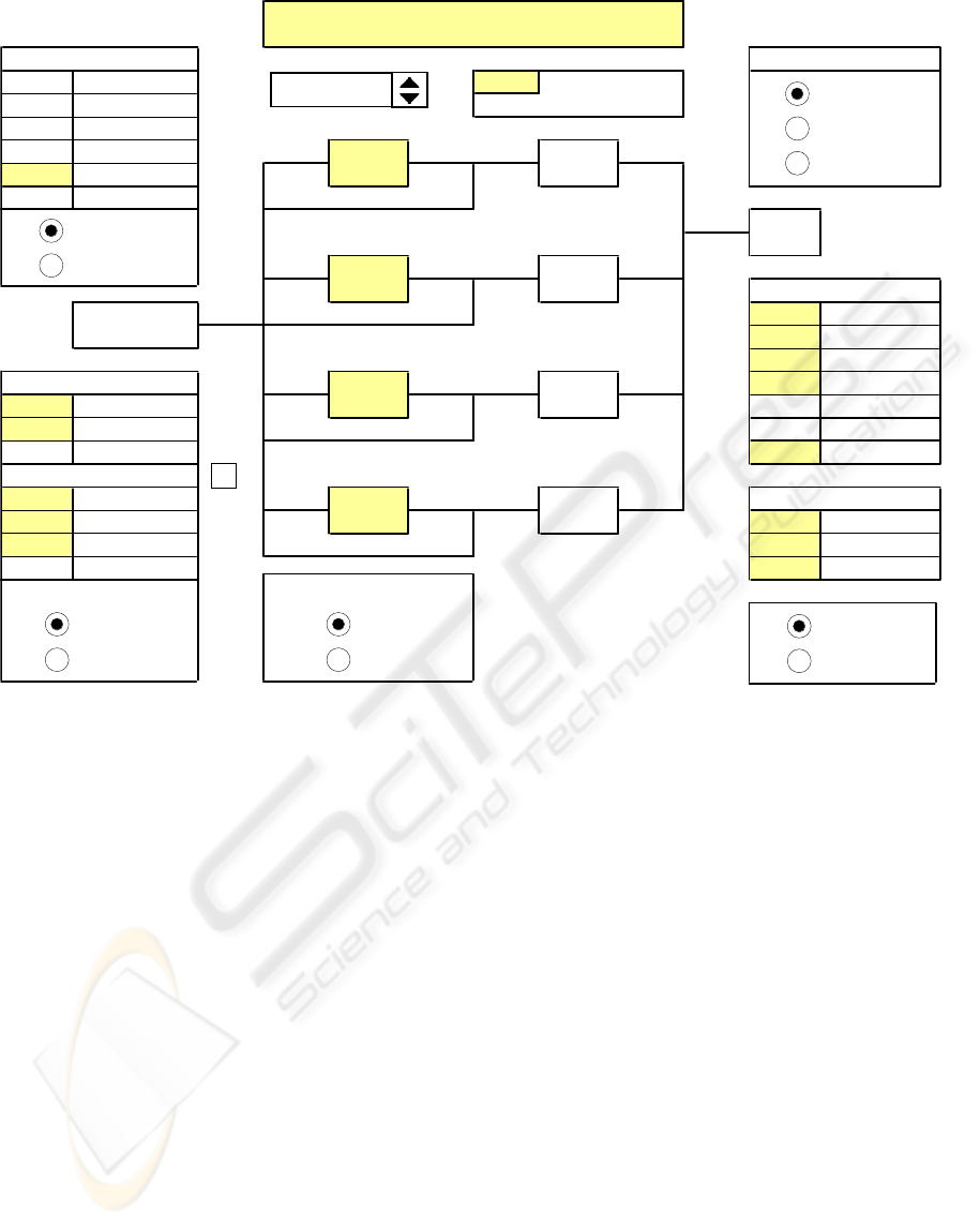
Figure 2 shows the Port “Specify” sheet. Settable
parameters are in yellow cells. In the example, the
ore arrives at 40 million tonnes per year, with a train
every six hours (generated in the Mine model). This
model explores a plan of up to four ship berths, with
each berth fed from a stockpile of nominated
capacity. Stockpiles can be fully Blended in Blended
Out (BIBO) or built First In First Out (FIFO).
Stockpile sizes are here set 240kt and 360kt. Train
and ship arrivals be equally spaced or random. The
cargo capacities distribution is specified. Each
incoming train can be direct loaded (with chosen
probability) to a ship, or sent to a stockpile, chosen
by a weighted composite of four criteria.
A “Progress” worksheet allows the system to be
tracked, at a chosen multiple of 6 hours, for a chosen
time range. This is useful for debugging, and also for
better understanding the system behaviour.
For each mineral, the “Cargoes” worksheet
graphs the cargo compositions varying around
target. For example, Figure 2 shows that the
“Process Capability” (the Tolerance divided by
twice the Standard Deviation) for Fe is 1.15.
The “Audit” worksheet reports the full simulation
history, with product flows and stockpile and ship
berth states for each time interval. Tonnage aspects
of the simulation history are plotted to aid
interpretation, and validate the parameter values
selected on a particular run.
58.0
58.2
58.4
58.6
58.8
59.0
0 120 240
+/- Ship Tolerance
95% Confidence
Days
Fe Cargoes
Process Capability=1.15 (2% Out of Tolerance)
Figure 2: The “Cargoes” Report.
ICEIS 2006 - ARTIFICIAL INTELLIGENCE AND DECISION SUPPORT SYSTEMS
302
6 CONCLUSIONS
As an example of the results, one simulation run
showed that to ship ore of acceptable quality at the
planned production rate required
1) 10% reduction of Mine short-term variability by
selective mining or pre-crusher stockpiling.
2) 30% priority to the use of Intelligent Stacking.
3) More accurate train composition estimates.
This solution was compared to installing blending
stockpiles at the mine and a cost/quality risk analysis
carried out. Without the simulation studies, many
capacity-related options such as this would have
been virtually impossible to evaluate.
The simulation models described are a valuable
aid to examine the effect on product chemical
quality of alternative potential development options,
to meet the potential capacity expansion required for
the rapidly increasing iron ore market.
The particular benefit in using Excel™ based
VBA simulation models is that it provides a familiar
mode of working for the company personnel,
enabling them efficiently to contribute domain
knowledge during running of the simulations,
without the assistance of the simulation developer.
In addition, the use of ExcelTM allows easy
interrogation of data and generation of reports.
REFERENCES
Everett, J. E., 1996, Iron ore handling procedures enhance
export quality.
Interfaces, 26/6, 82-94.
Everett J.E., 2001, Iron ore production scheduling to
improve product quality.
European Journal of
Operational Research,
129, 355-361.
Kamperman, M., Howard, T. and Everett, J.E., (2002),
Controlling product quality at high production rates.
Proceedings of the Iron Ore 2002 Conference, Perth,
Western Australia, 9-11 September 2002, ed. Holmes,
R., Australasian Inst. of Mining and Metallurgy:
Carlton, Victoria, ISBN 1 875776 94 X, 255-260.
Figure 3: The Port Model “Specify” Worksheet.
1
2048 Rakes, 12kt
890 Trains
224 Da
y
s 1 E
q
ual Interval
40.3 Max Mt/
y
ear
40.0 Mt/
y
ear
99% Train Slots
1
1 Random
0% 36 kt
0% 72 kt
0% 108 kt
0% 144 kt
70% Correct 100% 180 kt
30% Nei
g
hbou
r
Mean 180 kt
0% Random 96 hrs to 1st Car
g
o
FALSE
40% Low Tonna
g
e
30% Mine 0 Interval
(
hrs
)
30% Grade Estimate 0.00 Start
(
da
y)
0% Random 0.00 End
(
da
y)
1
11
As Stress BIBO 1 Track Stress
Stock
p
iles Shi
p
berths
Berth 2
240 kt
Shi
p
Car
g
oes
Shi
p
Arrival
Steady Cargo
Cargos
RandomBerth 1
Track GradeAs Grade
Show Train Rakes
Allocation Wei
g
ht
Track Pro
g
ress
LIFO
Build Stock
p
iles
240 kt Berth 4
360 kt
Run 1. 25% Direct Load
360 kt
Rake Grade Estimate
Trains
Equal Spaced
Direct Loadin
g
(
when
p
ossible
)
Berth 3
Ore Arrival
Menu
SIMULATION MODELLING OF IRON ORE PRODUCTION SYSTEM AND QUALITY MANAGEMENT
303
