
AdvWarp: A Transformation Algorithm for Advanced Modeling of Gas
Compressors and Drives
Anton Baldin
1
, Kl
¨
are Cassirer
1
, Tanja Clees
1,2
, Bernhard Klaassen
1
, Igor Nikitin
1
,
Lialia Nikitina
1
and Sabine Pott
1
1
Fraunhofer Institute for Algorithms and Scientific Computing, Schloss Birlinghoven, 53754 Sankt Augustin, Germany
2
Bonn-Rhine-Sieg University of Applied Sciences, Grantham-Allee 20, 53754 Sankt Augustin, Germany
Anton.Baldin, Klaere.Cassirer, Tanja.Clees, Bernhard.Klaassen, Igor.Nikitin, Lialia.Nikitina, Sabine.Pott
Keywords:
Complex Systems Modeling and Simulation, Non-linear Systems, Applications in Energy Transport.
Abstract:
Solving transport network problems can be complicated by non-linear effects. In the particular case of gas
transport networks, the most complex non-linear elements are compressors and their drives. They are described
by a system of equations, composed of a piecewise linear ‘free’ model for the control logic and a non-linear
‘advanced’ model for calibrated characteristics of the compressor. For all element equations, certain stability
criteria must be fulfilled, providing the absence of folds in associated system mapping. In this paper, we
consider a transformation (warping) of a system from the space of calibration parameters to the space of
transport variables, satisfying these criteria. The algorithm drastically improves stability of the network solver.
Numerous tests on realistic networks show that nearly 100% convergence rate of the solver is achieved with
this approach.
1 INTRODUCTION
In this paper, we continue the construction of globally
converging solver algorithm for stationary transport
network problems. The approach is based on condi-
tions of generalized resistivity formulated in our pre-
vious work (Clees et al., 2018a). Specifically for the
natural gas transport, the modeling of key elements,
the compressors, combines two parts, identified in gas
simulation community as ‘free’ and ‘advanced’ mod-
els. The ‘free’ model represents the control logic of
compressors, related to the fulfillment of goals, such
as the input/output pressure or flow. The ‘advanced’
model describes the individual physical characteris-
tics of compressors determined by calibration proce-
dure. The construction of the algorithm for advanced
modeling of compressors was started in (Clees et al.,
2018b), continued in (Baldin et al., 2020), and further
improved in the present paper.
The advanced model of compressors and drives
considers the space of calibration parameters such as
volumetric flow, revolution number, as well as vari-
ous energy characteristics. Although the representa-
tion of compressors and drives in this space is more
convenient for calibration, for solving transport net-
work problems it is more suitable to represent them
in the space, describing the main transport character-
istics, such as inlet and outlet pressures and mass flow.
It is important to fulfill the conditions of generalized
resistivity (Clees et al., 2018a), which means that the
flow must be an increasing function of the inlet pres-
sure and a decreasing function of the outlet pressure.
For the global convergence of the solver, this condi-
tion must be satisfied everywhere, including the exte-
rior of the working region, since the solver can wan-
der around there during the iterations.
In this work, to construct the element equation, an
improved pixel algorithm from (Clees et al., 2018b)
is used. A triangular grid (Baldin et al., 2020) is im-
plemented, which can be adaptively compressed in
places where higher resolution is required. Warping
of the grid will be performed in the solution loop
whenever the temperature or/and the gas composi-
tion change. This approach provides a simple con-
trol over the system resistivity by calculating the nor-
mals to the triangles. We tested the method on a vari-
ety of realistic examples and obtained nearly 100%
convergence of the solver. The approach enhances
our multi-physics network simulator MYNTS (Clees
et al., 2016).
Modeling of gas transport networks has been de-
scribed in detail in works (Mischner et al., 2011;
Baldin, A., Cassirer, K., Clees, T., Klaassen, B., Nikitin, I., Nikitina, L. and Pott, S.
AdvWarp: A Transformation Algorithm for Advanced Modeling of Gas Compressors and Drives.
DOI: 10.5220/0010512602310238
In Proceedings of the 11th International Conference on Simulation and Modeling Methodologies, Technologies and Applications (SIMULTECH 2021), pages 231-238
ISBN: 978-989-758-528-9
Copyright
c
2021 by SCITEPRESS – Science and Technology Publications, Lda. All rights reserved
231
Schmidt et al., 2015). The most numerous elements
in such networks are pipes, represented by a non-
linear friction law. In this law, the main dependence
is quadratic, and empirical approximations by Niku-
radse, Hofer, or Colebrook-White (Nikuradse, 1950;
Colebrook and White, 1937) are typically used. The
gas pressure and density are related by the equation
of state, for which also different approximations ex-
ist; commonly used are Papay, AGA8-DC92, GERG-
2008 (Saleh, 2002; CES, 2010; Kunz and Wagner,
2012). The balance of flows is described by linear
Kirchhoff equations. Finally, all the equations are
collected in a large non-linear system, which can be
considered as a particular type of non-linear program
(NLP). It can be solved by standard NLP solvers, such
as IPOPT, SNOPT, MINOS (W
¨
achter and Biegler,
2006; Gill et al., 2005; Murtagh and Saunders, 1978).
Our simulator also features an own solver, imple-
menting a stabilized Newton’s method with Armijo’s
rule (Kelley, 1995).
This paper is organized as follows. In Section 2
the transformation algorithm from the space of cali-
bration parameters to the space of transport variables
is presented. In Section 3 tests of the algorithm on
a number of realistic gas transport networks are de-
scribed and analyzed. In Section 4 the obtained re-
sults are summarized.
2 THE ALGORITHM
In the following, the general strategy as well as deci-
sive details of the novel algorithm are introduced.
Strategy: for stable representation of advanced
compressors and drives is based on the following
steps:
• eliminate all intermediate variables in the element
equation;
• represent the equation in the space of transport
variables;
• check monotonicity;
• use a monotone linear continuation outside of the
working region.
The sets of variables and the transformation be-
tween them will be described further. The mono-
tonicity condition is required for global convergence
of the solver algorithm and is described in (Clees
et al., 2018a). All element equations f (P
in
,P
out
,Q) =
0 should satisfy the following inequalities on their
derivatives:
∂ f /∂P
in
> 0, ∂ f /∂P
out
< 0, ∂ f /∂Q < 0, (1)
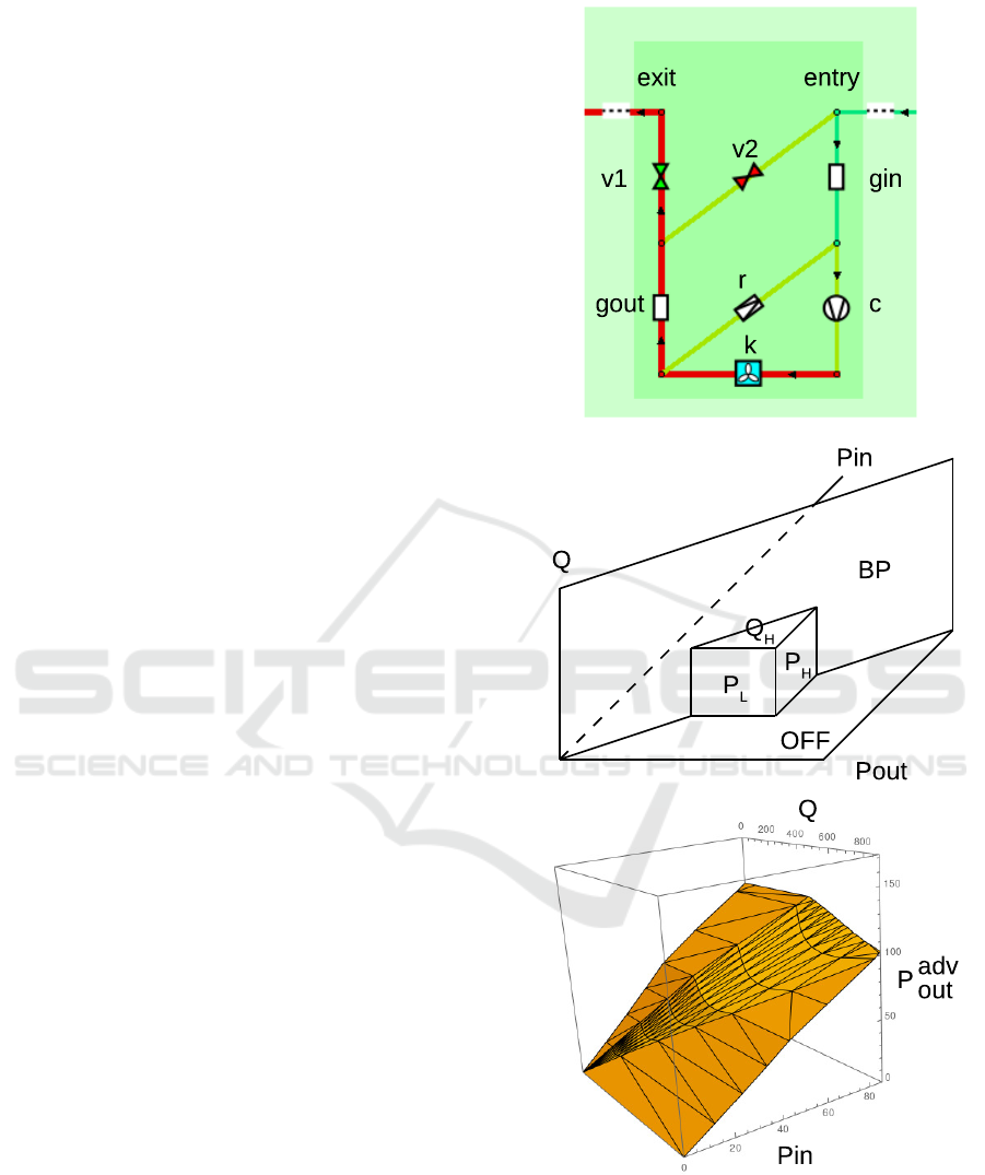
Figure 1: Modeling of compressors. On the top: the struc-
ture of compressor station. In the center: compressor el-
ement equation in transport variables, ‘free’ model. On
the bottom: ‘advanced’ model. Images from (Clees et al.,
2018a; Clees et al., 2018b; Baldin et al., 2020).
meaning that the element equation function should
monotonously increase w.r.t. P
in
and monotonously
SIMULTECH 2021 - 11th International Conference on Simulation and Modeling Methodologies, Technologies and Applications
232

decrease w.r.t. P
out
,Q.
The basic continuation formula is also presented
in (Clees et al., 2018a):
f (x
1
,...,x
n
) = f ( ˆx
1
,..., ˆx
n
)
+
n
∑
k=1
(min(x
k
− a
k
,0) +max(x
k
− b
k
,0)), (2)
ˆx
k
= min(max(x
k
,a
k
),b
k
).
It provides a continuation of the function of n argu-
ments, monotonously increasing w.r.t. every argu-
ment, from a bounding box specified by [a
k
,b
k
] limits
to the whole space, preserving this monotonous prop-
erty. For decreasing functions, coordinate reflections
can be used.
Structure: of the compressor station in its typical
one-unit configuration is shown in Figure 1 top. It
consists of the following elements: c – compressor, r
– bypass regulator, gin/gout – input and output resis-
tors, v1,2 – main and bypass valves, k – cooler. En-
try/exit identify standard input and output nodes. In
more complicated scenarios several units can be as-
sembled together in parallel or/and serial connection.
Transport Variables: Figure 1 center and bottom
show the element equation of compressor in the space
of transport variables. P
in,out
denote input and output
pressures, normally measured in bars. Q is a through-
put, standardly represented by mass flow Q
m
in kg/s.
With the known gas composition it can be converted
to molar flow Q
ν
in mol/s, or to normal flow Q
N
in
cubic meters of gas virtually decompressed to nor-
mal pressure and temperature, per second (often re-
expressed to thousands of such normal cubic meters
per hour). Special case is volumetric flow Q
vol
. It
is measured in m
3
/s at current conditions, and due to
compressibility of the gas depends on whether input
or output conditions are meant (input conditions are
taken by default).
Figure 1, central image, presents the free model.
The subscripts H,L indicate high and low control set-
tings, defining upper and lower limits on the pressures
and the flow; BP is open/bypass mode of compres-
sor P
in
= P
out
; OFF is the closed mode Q = 0. This
polyhedral surface, as all surfaces of this kind, can be
represented by max-min formula:
max(min( P
in
− P
L
,−P
out
+ P
H
,−Q +Q
H
), (3)
P
in
− P
out
,−Q) +ε(P
in
− P
out
− Q) = 0,
where the last term with small positive constant ε
serves regularization.
Figure 1 bottom presents advanced compressor
model. P
adv
out
(P
in
,Q) is output pressure of compressor
in the absence of control restrictions (also referred as
compressor in MAX mode). It is considered as a func-
tion of the input pressure and the flow. This function
represents the internal capability of compressor and
its drive. It is combined with free diagram as follows:
max(min( P
in
− P
L
,−P
out
+ P
H
,−Q +Q
H
,
−P
out
+ P
adv
out
(
ˆ
P
in
,
ˆ
Q)
+min(P
in
− P
adv
in,min
,0) +max(P
in
− P
adv
in,max
,0)
+min(−Q +Q
adv
max
,0) +max(−Q + Q
adv
min
,0) (4)
),P
in
− P
out
,−Q) +ε(P
in
− P
out
− Q) = 0,
ˆ
P
in
= min(max(P
in
,P
adv
in,min
),P
adv
in,max
),
ˆ
Q = min(max(Q, Q
adv
min
),Q
adv
max
),
here the second line represents the advanced surface,
inserted into the free formula; the next two lines pro-
vide linear continuation of this surface outside of the
bounding box; the last two lines define clamp func-
tions to the bounding box.
The advanced surface is triangulated, every trian-
gle is represented by own system of barycentric coor-
dinates. For this purpose, on the plane (P
in
,Q) = (x,y)
the vertices of triangle {v
1
,v
2
,v
3
} are defined. The
point on triangle is then defined as
∑
i
w
i
v
i
= (x,y),
∑
i
w
i
= 1. The system can be solved for the weights
w
i
(x,y) by linear formulae w
i
(x,y) = c
0i
+ c
xi
x + c
yi
y,
with 3 constants (c
0i
,c
xi
,c
yi
) per w
i
precomputed.
One formula can be spared using w
3
= 1 − w
1
− w
2
.
The point belongs to triangle, when all weights are
non-negative w
i
≥ 0.
The third coordinate P
out
= z is found by one more
linear formula z(x,y) =
∑
i
w
i
(x,y)z
i
. Altogether 9 co-
efficients (equivalent to 3 nodes x 3 coordinates) are
precomputed. Explicit lengthy formulae for barycen-
tric coordinates can be found in (Baldin et al., 2020).
Finally, a function is implemented, searching for a tri-
angle on xy-plane and evaluating z-coordinate and its
xy-derivatives. The derivatives can be directly used to
check monotonicity condition:
−P
out
+ P
adv
out
(P
in
,Q) = 0, (5)
∂P
adv
out
/dP
in
> 0, ∂P
adv
out
/dQ < 0.
Equivalently, these conditions can be reformulated in
terms of normals to triangles, which all should point
to the octant (P
in
,P
out
,Q) = (+,−,−).
Internal Variables: Density ρ is defined as
monotonously increasing function of pressure P us-
ing equations of state (EOS), involving also the mo-
lar mass µ, the temperature T and the compressibil-
ity factor z. Different analytic or numerical EOS
can be used, e.g., Papay (Saleh, 2002), AGA8-DC92
AdvWarp: A Transformation Algorithm for Advanced Modeling of Gas Compressors and Drives
233
(CES, 2010), GERG-2008 (Kunz and Wagner, 2012).
The volumetric flow relative to input conditions is ex-
pressed via mass flow and density as Q
vol
= Q/ρ
in
.
The revolution number rev and torque M
t
describe the
rotation of the engine. There are also energetic quan-
tities characterizing compressors and drives: H
ad
–
increase of adiabatic enthalpy, η
ad
– adiabatic effi-
ciency, Perf – performance power.
Transformation: consists of a sequence of non-
linear maps:
(Q
vol
,rev)
1
→ (H
ad
,η
ad
,Perf
max
)
2
→ (6)
→ (ρ
in
,H
ad
,Q)
3
→ (P
in
,P
out
,Q).
Step 1: standard 1D quadratic and 2D biquadratic
models from (Clees et al., 2018b):
H
ad
= (1, rev,rev
2
) · A · (1,Q
vol
,Q
2
vol
)
T
,
η
ad
= (1, rev,rev
2
) · B · (1,Q
vol
,Q
2
vol
)
T
, (7)
Perf
max
= (1, rev,rev
2
) · D
T
,
where A,B are constant 3x3 matrices and D is a
constant 3-vector filled by calibration coefficients.
Perf
max
is the maximal performance power provided
by the drive at the given revolution number.
Step 2: temperature and gasmix independent models:
Q = Perf
max
η
ad
/H
ad
, ρ
in
= Q/Q
vol
, (8)
Step 3: temperature and gasmix dependence:
α = (κ −1)/κ, γ = RT
in
/µ,
P
in
= EOS
inv
(ρ
in
), z
in
= P
in
/(γρ
in
), (9)
P
out
= P
in
(H
ad
α/(γz
in
) + 1)
1/α
,
where κ is the adiabatic exponent, R is universal gas
constant; the equation of state ρ = EOS(P) is inverted
to define P
in
; the universal gas law P = ρRT z/µ is re-
solved w.r.t. z; then H
ad
definition from (Clees et al.,
2018b) is resolved w.r.t. P
out
.
All equations are given in SI-units, practically
conversion factors should be applied for the transfor-
mations W/kW/MW, bar/Pa etc.
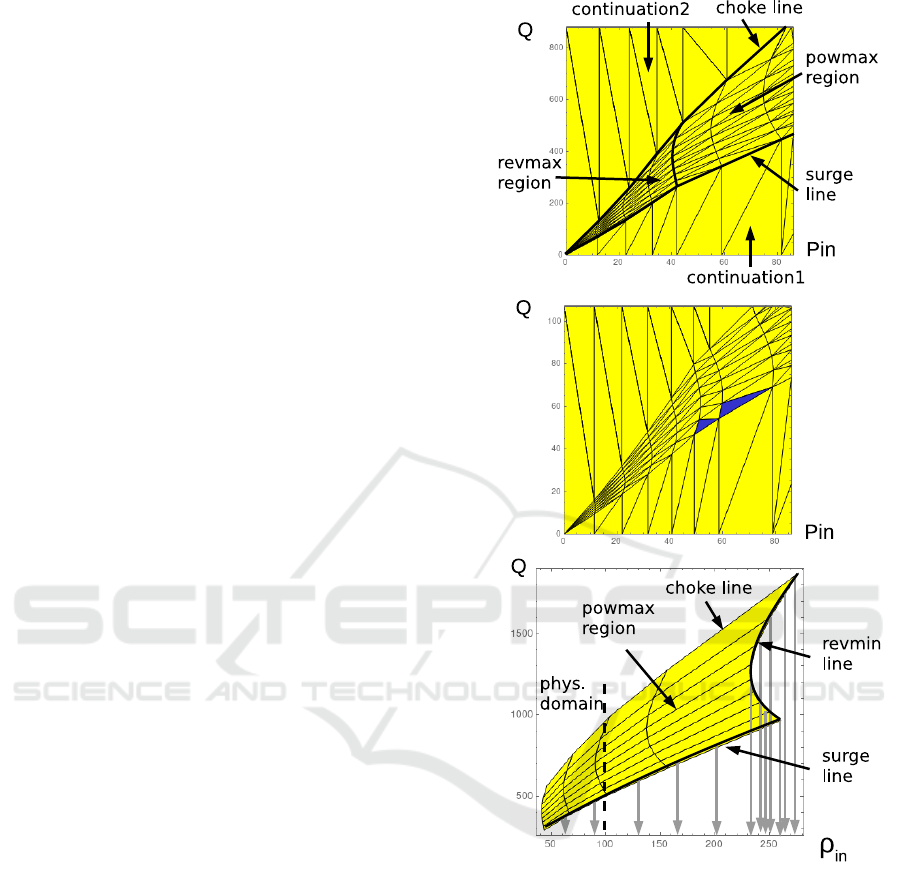
Regions: of the advanced surface are shown in
Figure 2 top. The described transformations are
used to construct the most important powmax re-
gion, where the performance of compressor is re-
stricted solely by the power of its drive. It is bounded
by revmin/revmax lines and Q
vol,min
/η
min
lines (also
called surge line and choke line). Here revmin and
Figure 2: Details of compressor diagrams. On the top: re-
gions of the advanced surface in (P
in
,Q) projection. In the
center: problems with monotonicity detected (blue trian-
gles). On the bottom: the fold on revmin line.
revmax are given constants. Surge line is defined as
Q
vol,min
(rev) = max(Q
(1)
vol,min
,Q
(2)
vol,min
,0),
Q
(1)
vol,min
= (1, rev,rev
2
) ·C
T
, (10)
Q
(2)
vol,min
= arg max
Qvol
H
ad
(Q
vol
,rev),
Q
(1)
vol,min
is given as 1D quadratic model with a cali-
bration 3-vector C; the condition Q
vol
≥ Q
(2)
vol,min
de-
fines a physical decreasing branch of quadratic de-
pendence of H
ad
on Q
vol
at fixed rev; the outflow
SIMULTECH 2021 - 11th International Conference on Simulation and Modeling Methodologies, Technologies and Applications
234
condition Q
vol
≥ 0 is also enforced. Choke line
η
ad
(Q
vol,max
,rev) = η
min
with a given constant η
min
is
solved w.r.t. Q
vol,max
(rev). Generally it is a quadratic
equation with two roots; the maximal root is taken.
The region between revmin/revmax and surge/choke
lines is resampled to N
rev
× N
η
grid.
Revmax region: rev = revmax side is taken and in
(ρ
in
,Q) projection proportionally scaled to the origin.
Then it is mapped to the final (P
in
,Q) coordinates by
the inverse EOS transformation above.
Continuation regions 1 and 2 go downwards and
upwards in the (ρ
in
,Q) projection, respectively, till
the limits of the bounding box. H
ad
values in these
continuations are kept constant.
P
out
-coordinate in (9) lifts the whole construc-
tion to 3D space (P
in
,P
out
,Q), where the final surface
is represented by triangulation. Orientation of nor-
mals allows to check monotonicity conditions for ev-
ery triangle. Figure 2 center indicates problems with
monotonicity (blue triangles). These problems hap-
pen rarely and require a slight local adjustment of the
diagram to satisfy the global convergence criterion.
In general, the revmin side of the powmax patch
has a fold, shown in Figure 2 bottom. Physically, on
the surge and revmin lines, a bypass regulator opens
in compressor station (r in Figure 1 top). It redirects
a part of the flow to circulate through the compres-
sor, preventing the compressor from going outside of
the working region (Q
vol
< Q
vol,min
, rev < revmin). In
our diagrams, total Q passing through the compres-
sor and its bypass regulator is continued downwards
from these lines. This continuation generally creates a
fold, producing multiple solutions and degeneracy of
the Jacobi matrix. Fortunately, for most of the cases,
this fold is located beyond the physical domain of ρ
in
or P
in
and can be safely ignored. For extra safety, we
define a ρ
in,max
value, cutting off the fold and restrict-
ing the patch by this value.
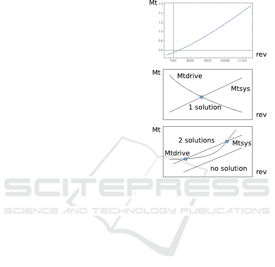
The other problematic case is displayed in Fig-
ure 3 top. It corresponds to the increasing torque
dependence M
t
(rev) = Perf
max
/rev. If the drive is
joined with a generic resistive load, M
t,sys
(rev) =
c
0
+ c
1
rev for dry and viscous friction, or other in-
creasing M
t,sys
(rev) dependence, the stable intersec-
tion is ensured only when M
t,drive
(rev) is decreasing,
Figure 3 center. Otherwise one can find such resis-
tive system that none or multiple intersections exist,
Figure 3 bottom. In this case multiple solutions or no
solution exist for the whole network problem. Such
problematic behavior is present in some electric en-
gines (E-drives). The computations show that in this
case the monotonicity conditions are violated in most
of the diagram. The solution we have taken so far
is to replace the actual M
t,drive
(rev) dependence with
Figure 3: Dependence of torque on revolution number.
On the top: problematic case with increasing M
t
(rev) de-
pendence. In the center: stable intersection of increas-
ing M
t,sys
(rev) and decreasing M
t,drive
(rev). On the bot-
tom: no intersection or multiple intersections for increasing
M
t,drive
(rev).
a weakly decreasing function that limits the real de-
pendence from below (conservative), above (overes-
timation), or reproduces it on average. In practice, a
constant M
t,drive
can be used here, since the regular-
ization in the control equation removes all marginal
degenerations in the system.
The described transformation procedure is applied
sequentially for all compressor-drive pairs in the net-
work, as shown in Figure 4. Steps 1 and 2 of the
transformation are performed once, in precomputa-
tion mode. The monotonous decrease of M
t
(rev),
regularity of surge and choke lines, absence of folds
on 2D diagrams is visually controlled. Step 3 of the
transformation is applied repeatedly during the so-
lution procedure, every time when the temperatures
or/and gas composition changes. This step is just
a monotonous remapping ρ
in
→ P
in
according to the
current EOS, not violating the verified monotonicity
conditions.
AdvWarp: A Transformation Algorithm for Advanced Modeling of Gas Compressors and Drives
235
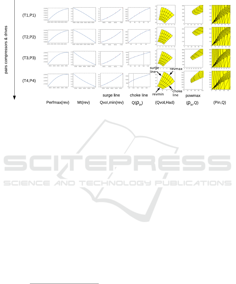
Figure 4: Construction of advanced representation for all compressor-drive pairs in the network.
Station Resistors: shown by gin/gout in Figure 1
top, the resistors typically support constant pressure
drops (REPD) on entry and exit of compressor sta-
tion. They lead to trivial modification of the control
equation (4), where in the first line P
in/out
represent
the pressure in entry/exit nodes, while in the rest of
the formula P
in/out
are replaced with the pressure at
inlet/outlet of the compressor. These values differ by
the given pressure drops on station resistors.
Ambient Temperature Dependence: compressor
drives often possess an own dependence on ambient
temperature, defined by biquadratic model:
Perf
max
= (1, rev,rev
2
) · D · (1,T
amb
,T
2
amb
)
T
, (11)
used instead of (7). Here D is 3x3 calibration ma-
trix and T
amb
is absolute or relative temperature, with
the corresponding recomputation. Note that the ac-
tual use of Perf
max
in step 2 of the transformation is
a linear formula (8). As a result, the following lin-
ear algorithm can be used for precise account of T
amb
-
dependence. The step 2 precomputation is performed
for three different temperature values T
amb,i
, produc-
ing three 2-vectors v
i
= (ρ
in
,Q)
i
. Then, in step 3,
three weights are computed, defined by
w
1
=
(T
amb
− T
amb,2
)(T
amb
− T
amb,3
)
(T
amb,1
− T
amb,2
)(T
amb,1
− T
amb,3
)
(12)
and the cyclic permutation of indices. Then the vec-
tor v is computed as the weighted average v =
∑
i
w
i
v
i
and the result is passed to step 3 of the generic com-
putation. In this way, the variation of T
amb
in partic-
ular scenario can be performed without repeating the
steps1,2 in the chain.
3 NUMERICAL TESTS
The described algorithm has been tested on a number
of real-life gas networks. Parameters of the test net-
works are given in Table 1. The number of elements is
given before applying topological cleaning procedure,
described in (Clees et al., 2018b). This procedure
removes trivial elements, such as valves, shortcuts,
short pipe segments, and can significantly reduce the
size of the network in certain cases. While the trans-
port networks mainly consist of pipes with a nearly
quadratic friction law, their computational complex-
ity is defined by the most non-linear elements, namely
compressors and regulators. In the networks, there are
two types of supply nodes, the ones with a pressure
setpoint (Pset) and the ones with an inflow setpoint
(Qset < 0). Many outflow nodes (Qset > 0) exist,
representing the large number of gas consumers in the
network.
The small and medium size networks are pre-
sented in Figure 5. Network N1 has 100 nodes and
111 edges, while ME has 437 nodes and 482 edges
and possesses a more complex topology. In addition,
we use a set of 85 large networks received from our
industrial partner for benchmarking. They are sub-
divided to L- and H-type denoting gas with low and
high calorific value. Although the calorific value it-
self has no influence on the convergence properties,
the L-networks contain considerably less compres-
sors and are topologically more simple than their H-
counterparts. As a result, L-networks typically pos-
sess better convergence then the H-ones.
The test networks were subjected to the solver
procedures of two types. One used the ‘old’ type
SIMULTECH 2021 - 11th International Conference on Simulation and Modeling Methodologies, Technologies and Applications
236

Table 1: Parameters of test networks.
network nodes edges pipes compressors regulators Psets Qsets
N1 100 111 34 4 4 2 3
ME 437 482 370 20 24 3 164
N85/L 3232-3886 3305-3974 2406-2835 1-7 59-77 6-7 625-843
N85/H 2914-3818 2989-3952 1498-1937 16-42 59-107 5-9 328-505
Figure 5: Test networks N1 and ME.
of the compressor modeling, where all intermediate
variables were present and constrained by the corre-
sponding equations. The other one used the ‘new’
type, with intermediate variables eliminated and the
problem formulated completely in terms of the trans-
port variables. The convergence results are shown in
Table 2. While the old procedure was sufficiently sta-
ble to process simple N1 and ME networks, as well as
L-type N85 networks, it diverged in the half of H-type
N85 networks. Our main achievement is that the new
procedure converged in our tests in 100% of cases,
also in the most complex N85/H-type ones.
It should be noted, however, that in spite of the
theoretical guarantee for the convergence of the al-
gorithm, the control equations (3) and (4) contain
problematic marginally degenerate terms. They cor-
respond to the faces of the ’free’ diagram (Figure 1,
center), with normals directed exactly along coordi-
nate axes. On such faces, some derivatives in (1) van-
ish and the whole network problem degenerates. Reg-
ularizing the ε-term in the control equations formally
removes this singularity. However, precise physical
modeling requires ε to be as small as possible while
for numerical stability larger values of ε are prefer-
able. In our applications, a compromise value in the
range ε = [10
−6
,10
−3
] is selected.
As a result of the marginally singular problem
statement, the solution procedure cannot be started
Table 2: Results.
test total converged
networks num. old new
N1 1 1 1
ME 1 1 1
N85/L 23 23 23
N85/H 62 31 62
from an arbitrary point, as it should be possible for
the absolutely stable globally convergent algorithm.
It still requires empirics in the definition of a start-
ing point, for which we use a ‘gradual sophistication’
strategy. It starts from ‘forced’ goals of compressors
and regulators and proceeds via ‘free’ to ‘advanced’
modeling. We have found that the solution procedure
can randomly diverge under variations of the problem
settings. It happens rarely, by our experience in ∼ 1%
of cases. In these special cases the adjustment of ε
value, global per network or local per problematic el-
ement, may help.
AdvWarp: A Transformation Algorithm for Advanced Modeling of Gas Compressors and Drives
237

4 CONCLUSIONS
In this paper, the advanced modeling of gas compres-
sors and their drives is considered. The approach
is based on the transformation of a system from the
space of calibration parameters to the space of trans-
port variables. In the solution loop, the transforma-
tion is readjusted whenever the temperature or/and the
gas composition in the network change. The transfor-
mation satisfies stability criteria providing the global
convergence of the solution procedure. For the 87 test
cases considered, 100% convergence rate is achieved.
The remaining problem is the presence of the
marginally degenerate terms in the control equation of
compressors and regulators. In our current approach,
we regularize these terms with a small positive param-
eter, whose value is balanced between physical preci-
sion and numerical stability of the modeling. Other
approaches have to be tested, in particular, enhancing
the system by dynamic behavior and studying the sta-
bility of the integrator of the corresponding system of
differential algebraic equations.
Our further plans also include the consideration of
‘generic’ modeling, intermediate between ‘free’ and
‘advanced’, as well as a special analytically solvable
case of piston compressors.
ACKNOWLEDGMENT
We acknowledge the support of the German Federal
Ministry for Economic Affairs and Energy, project
BMWI-0324019A, MathEnergy: Mathematical Key
Technologies for Evolving Energy Grids.
REFERENCES
Baldin, A. et al. (2020). Topological Reduction of Sta-
tionary Network Problems: Example of Gas Trans-
port. International Journal On Advances in Systems
and Measurements, 13:83–93.
CES (2010). DIN EN ISO 12213-2: Natural gas – Calcula-
tion of compression factor. European Committee for
Standardization.
Clees, T. et al. (2016). MYNTS: Multi-phYsics NeTwork
Simulator. In SIMULTECH 2016, July 29–31, 2016,
Lisbon, Portugal, pages 179–186. SCITEPRESS.
Clees, T. et al. (2018a). Making Network Solvers Glob-
ally Convergent. Advances in Intelligent Systems and
Computing, 676:140–153.
Clees, T. et al. (2018b). Modeling of Gas Compressors and
Hierarchical Reduction for Globally Convergent Sta-
tionary Network Solvers. International Journal On
Advances in Systems and Measurements, 11:61–71.
Colebrook, C. F. and White, C. M. (1937). Experiments
with Fluid Friction in Roughened Pipes. Mathemati-
cal and Physical Sciences, 161:367–381.
Gill, P. E. et al. (2005). SNOPT: An SQP algorithm for
large-scale constrained optimization. SIAM Review,
47(1):99–131.
Kelley, C. T. (1995). Iterative Methods for Linear and Non-
linear Equations. SIAM, Philadelphia.
Kunz, O. and Wagner, W. (2012). The GERG-2008 wide-
range equation of state for natural gases and other
mixtures: An expansion of GERG-2004. J. Chem.
Eng. Data, 57:3032–3091.
Mischner, J. et al. (2011). Systemplanerische Grundla-
gen der Gasversorgung. Oldenbourg Industrieverlag
GmbH.
Murtagh, B. and Saunders, M. (1978). Large-scale lin-
early constrained optimization. Mathematical Pro-
gramming, 14:41–72.
Nikuradse, J. (1950). Laws of flow in rough pipes. NACA
Technical Memorandum 1292, Washington.
Saleh, J. (2002). Fluid Flow Handbook. McGraw-Hill.
Schmidt, M. et al. (2015). High detail stationary optimiza-
tion models for gas networks: model components. Op-
timization and Engineering, 16(1):131–164.
W
¨
achter, A. and Biegler, L. T. (2006). On the implemen-
tation of an interior-point filter line-search algorithm
for large-scale nonlinear programming. Mathematical
Programming, 106(1):25–57.
SIMULTECH 2021 - 11th International Conference on Simulation and Modeling Methodologies, Technologies and Applications
238
