Using Syntactic Similarity to Shorten the Training Time of Deep

Learning Models using Time Series Datasets: A Case Study

Silvestre Malta

1,2 a

, Pedro Pinto

2,3 b

and Manuel Fern

andez Veiga

1 c

University of Vigo and AtlanTTic Research Center, Spain

ADiT-Lab, ESTG - Instituto Polit

ecnico de Viana do Castelo, Portugal

INESC TEC, R. Dr. Roberto Frias, Porto, Portugal

Keywords:

Neural Networks, Machine Learning, NLP, LSTM, RNN, GRU, CNN, Word2Vec, Mobility Prediction,

Training Time Optimization.

Abstract:

The process of building and deploying Machine Learning (ML) models includes several phases and the training

phase is taken as one of the most time-consuming. ML models with time series datasets can be used to predict

users positions, behaviours or mobility patterns, which implies paths crossing by well-deﬁned positions, and

thus, in these cases, syntactic similarity can be used to reduce these models training time. This paper uses

the case study of a Mobile Network Operator (MNO) where users mobility are predicted through ML and the

use of syntactic similarity with Word2Vec (W2V) framework is tested with Recurrent Neural Network (RNN),

Gate Recurrent Unit (GRU), Long Short-Term Memory (LSTM) and Convolutional Neural Network (CNN)

models. Experimental results show that by using framework W2V in these architectures, the training time

task is reduced in average between 22% to 43%. Also an improvement on the validation accuracy of mobility

prediction of about 3 percentage points in average is obtained.

1 INTRODUCTION

In the past few years, due to the availability of large

datasets and exponential increase of computational

power, Machine Learning (ML) has been used in

ﬁelds such as self driving cars, speech and image

recognition, medical diagnosis, cybersecurity, etc.

However, to take the advantages of ML, a set of tasks

must be accomplished to deploy these algorithms.

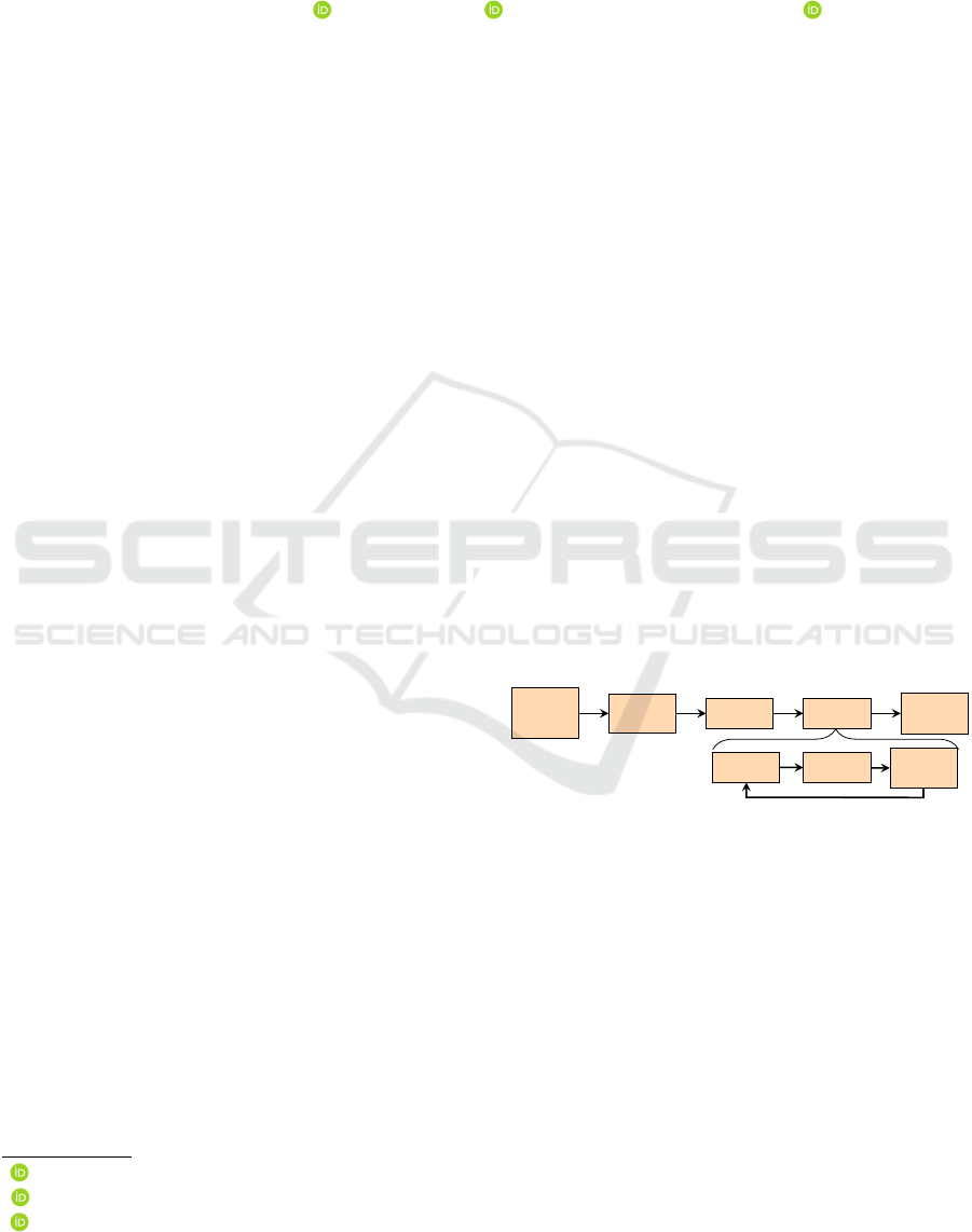
These tasks can be organized as in Fig. 1. Initially

a ML problem and a solution must be proposed. The

second task is to collect and transform data to feed the

model. Then, it is necessary to choose a model, train it

and evaluate the results. Finally, there is a prediction

and deployment task. Train a model major task can be

grouped in different sub-tasks: model training, model

evaluation and hyperparameter tuning. After training

the model and evaluating the results, a hyperparame-

ters tuning task is needed as each ML problem is dif-

ferent. These training sub-tasks must be repeated un-

til the optimum set of hyperparameters is determined

https://orcid.org/0000-0002-5274-3733

https://orcid.org/0000-0003-1856-6101

https://orcid.org/0000-0002-5088-0881

to minimize the error and have predictions as close as

possible to actual values.

Deﬁne

a ML

problem

and propose

a solution

Collect

and

Transform

Data

Choose

Model

rain a

Model

rain

aluate

Hyper

parameter

Tuning

ediction

and De-

ployment

Figure 1: ML tasks.

This paper focuses on speciﬁc ML problems in-

volving mobility prediction, i.e. intended to predict

the position of an object or person within a path,

useful for epidemic control, intelligent transporta-

tion management, urban planning, location-based ser-

vices, management of cellular network resources, etc.

Thus, a particular case study is assumed where a

Mobile Network Operator (MNO) intends to pre-

dict user mobility. This ML problem uses the mo-

bility data of a set of users passing through mo-

bile cells of a MNO and predicts the next cell in a

path. MNOs collect relevant data from their networks,

systems and users. The data collected from users

may be obtained from smart phone sensors, Global

Positioning Systems (GPS), Global System for Mo-

Malta, S., Pinto, P. and Veiga, M.

Using Syntactic Similarity to Shorten the Training Time of Deep Learning Models using Time Series Datasets: A Case Study.

DOI: 10.5220/0010515700930100

In Proceedings of the 2nd International Conference on Deep Learning Theory and Applications (DeLTA 2021), pages 93-100

ISBN: 978-989-758-526-5

bile Communications (GSM), social-media apps with

geo-spacial recording, location estimation extracted

using wireless Local Area Network (LAN) proto-

cols or Radio Frequency Identiﬁcation (RFID) (Jeung

et al., 2014) which generate datasets such as CRAW-

DAD (Kotz et al., 2005) or GeoLife (Zheng et al.,

2011). The dataset used in this case study was Mo-

bile Data Chalenge (MDC) that has been provided by

Nokia Research Center and Idiap (Kiukkonen et al.,

2010)(Laurila et al., 2013). Datasets that have time

series characteristics, i.e., each event has time period

attached, can be trained by Recurrent Neural Net-

works (RNNs) as they allow to model temporal dy-

namic behavior or natural language. Gate Recurrent

Unit (GRU) and Long Short-Term Memory (LSTM)

are modiﬁed versions of RNN giving them the ability

to extend the data memory, by using internal mech-

anisms called gates that can regulate the ﬂow of in-

formation, fostering its results when predicting time

series data.

As stated in (Miranda and Von Zuben, 2015), from

all the ML tasks the model training is one of the most

time-consuming. Since the scenario intends to pre-

dict mobility in a MNO, the user’s path composed by

cells can be converted into a sentence composed by

words and, therefore, ML can be taken as an Nat-

ural Language Processing (NLP) problem that can

be solved using word embedding frameworks such

as Word2Vec (W2V) (Mikolov et al., 2013). W2V

receives text as input and outputs a set of feature

vectors representing the words in a numerical form.

Words with similar context have similar embeddings

and thus, they are close in the resulting vector space.

This paper proposes the use of W2V to reduce the

training time of a ML mobility prediction problem. A

set of four architectures combining ML models based

on RNN, GRU, LSTM and Convolutional Neural Net-

work (CNN) were deﬁned and trained with and with-

out W2V, and their training time and mobility accu-

racy was obtained and compared.

The experimental results show that by using the

pre-trained weights obtained from W2V, models

present a shorter training time in average and an im-

provement on validation accuracy when predicting

next cell ID where user will be connecting to.

2 RELATED WORK

There are research works focused in reducing the

time to build and deploy ML models. As stated

in (Shi et al., 2017), to address the huge computa-

tional challenge in Deep Learning (DL), many tools

have been developed to exploit hardware features

such as multi-core CPUs and many-core GPUs to

shorten the training and inference time, however those

tools exhibit different features and running perfor-

mance when they train different types of deep net-

works on different hardware platforms, making it dif-

ﬁcult for end users to select an appropriate pair of

software and hardware. The authors present a bench-

mark with tree major types of Deep Neural Network

(DNN): Fully Connected Feed-Forward Neural Net-

works (FCNs), CNNs and RNNs, comparing their

running performance with four state-of-the-art GPU-

accelerated tools: Caffe (Jia et al., 2014), CNTK (Mi-

crosoft Azure, 2017), TensorFlow (Abadi et al., 2015)

and Torch (Collobert et al., 2008). They concluded

that (1) in general, the performance does not scale

very well on many-core CPU; (2) no obvious single

winner was observed on CPU-only platforms; and (3)

all tools can achieve signiﬁcant speedup using con-

temporary GPUs. In (Reif et al., 2011) the authors

presented a method for predicting the run-time of a

classiﬁcation algorithm comparing the computation

time of several algorithms. In (Kretowicz and Biecek,

2020) the authors deeply test to ﬁnd the best defaults

values of hyperparameters on a set of different ML

algorithms, and computational learning time was also

benchmarked to ﬁnd best hyperparameter conﬁgura-

tion. In (Miranda and Von Zuben, 2015) authors de-

veloped a method for pre-training neural networks

that can decrease the total training time for a neural

network while maintaining the ﬁnal performance by

partitioning the training task in multiple training sub-

tasks with sub-models.

RNNs were designed for classiﬁcation predic-

tion problems along temporal sequences of data and

GRUs and LSTMs derived from the RNN architec-

ture. In (Wickramasuriya et al., 2017) authors pro-

pose RNNs models to train sequences of Received

Signal Strength (RSS) values to predict Base Station

(BS) associations with the end user. In (Yang et al.,

2018) authors propose a model based on RNN and

GRU that can joint social networks and mobile tra-

jectories to capture both short-term and long-term se-

quential contexts. In (Wang et al., 2018) authors pro-

pose an intelligent dual connectivity mechanism for

mobility management using an LSTM algorithm to

deal with more frequent handovers in ﬁfth-generation

(5G) mobile communication system due to Ultra-

dense network deployment. CNN models have been

shown to be effective for NLP in semantic parsing. In

(Yih et al., 2014) authors propose a semantic parsing

framework where a ﬁrst layer based on CNN, projects

each word within a context window to a local contex-

tual feature vector, so that semantically similar word-

n-grams are projected to vectors that are close to each

DeLTA 2021 - 2nd International Conference on Deep Learning Theory and Applications

other in the contextual feature space. In (Kim, 2014)

authors used simple CNN on top of pre-trained word

vectors for sentence-level classiﬁcation tasks. Re-

sults show that their baseline model with all randomly

initialized words did not performed well on its own,

while with the use of pre-trained vectors, performance

gains where obtained. LSTM, CNN and GRU have

been used in (Tang et al., 2015), to encode the intrin-

sic relations between sentences in the semantic mean-

ing of a document. They modelled documents repre-

sentation in two steps. Firstly using CNN or LSTM

to produce sentence representations from word rep-

resentations and secondly the GRU is used to adap-

tively encode semantics of sentences and their inher-

ent relations in document representations. These rep-

resentations are used as features to classify the senti-

ment label of each document. Results show that GRU

outperforms standard RNN in document modeling for

sentiment classiﬁcation.

As explained in (Hashimoto et al., 2015),

embedding-based models are proposed to tackle clas-

siﬁcation problems using lexical relation-speciﬁc fea-

tures on a large unlabeled corpus, allowing to explic-

itly incorporate relation-speciﬁc information into the

word embeddings. In (Zayats and Ostendorf, 2018)

the authors proposed a novel approach for modeling

threaded discussions on social media using a graph-

structured bidirectional LSTM using W2V lexical ca-

pabilities in experiments with a task of predicting

popularity of comments in forum discussions. In (Fan

et al., 2018) the authors used W2V to build their

Loc2vec model, which provided contextual features

to CNN and bidirectional LSTM networks to predict

next location of vehicles.

The works surveyed do not explore syntactic simi-

larity embeddings techniques applied to cell paths us-

ing RNN, GRU, LSTM or CNN, in order to reduce

training time.

3 METHODOLOGY

Assuming that the case study is a ML model to pre-

dict mobility, and that training task is one of the most

time consuming task, MDC dataset was selected to be

used in a set of ML architectures to assess training

time and mobility prediction accuracy.

MDC dataset includes data from smartphones of

185 volunteers collected over 18 months in the Swiss

Geneva lake region. MDC collected user logs with a

total of 99166 unique cell towers which permitted to

obtain the identiﬁcation from the BSs that each user

was connected in his daily trajectory. The MDC was

anonymized and each user has his unique location set,

thus, it is not possible to correlate data from multi-

ple users. Then, the focus was set on individual loca-

tion trajectory data, extracting features as cell ID and

time, and with the repeated contiguous cell IDs on

the historical movements removed. As feature for the

model, cell ID has been chosen to transform this iden-

tiﬁer into a unique string, allowing to build a set of

phrases which were used as input to W2V. As stated

in (Gonz

alez et al., 2008), each individual is char-

acterized by a time-independent travel characteristic,

having a high degree of temporal and spatial regular-

ity there is a signiﬁcant probability to return to a few

highly frequented locations. As presented in Table 1,

9 users were randomly chosen from MDC dataset and

divided in 3 subsets range, each user dataset contains

trajectories being the size deﬁned by Number of Cells

(#Cells) that represents the number of cells. The vari-

able Number of Unique Cells (#UCells) was deﬁned

to represent unique cells contained in each user sub-

set dataset, e.g. a path containing a cell trajectory with

-C

has a #Cells of 4 and a #UCells of 3 and

the variable Number of Paths (#Paths) represents the

#Paths per user subset dataset.

As MDC dataset has approximately 18 months of

mobility data for each user, time is implicit in each in-

put data variable used in the learning process and the

output variable is treated as a classiﬁcation problem,

where the cell ID predicted is one among all the cell

IDs used during each user trajectory. To preserve the

order of cell sequences and tackle the user mobility

as a time series data problem, each user dataset was

divided in samples paths of 5 cells. The sliding win-

dow transformation technique presented in Fig. 2 was

used to divide trajectories in smaller paths were: (1)

X represents 5 time steps containing a cell ID in each

time step, and (2) Y represents the next predicted cell

ID. As of W2V input data, each user subset dataset

is divided in sliding windows that are handled as sen-

tences and each sentence is composed of cell IDs that

are handled as words.

X Y

[34, 76, 96, 34, 11] [50]

[76, 96, 34, 11, 50] [23]

[96, 34, 11, 50, 23] [10]

[34, 11, 50, 23, 10] [96]

[11, 50, 23, 10, 96] [??]

Figure 2: Division of trajectory in sliding windows of 5

cells per path.

A set of ML architectures were designed to be

tested and treat sequential data, and therefore, they

based on the following models: RNN, GRU, LSTM,

and hybrid CNN+LSTM. The four designed architec-

tures are presented in Fig. 3 and consist of Simple Re-

Using Syntactic Similarity to Shorten the Training Time of Deep Learning Models using Time Series Datasets: A Case Study

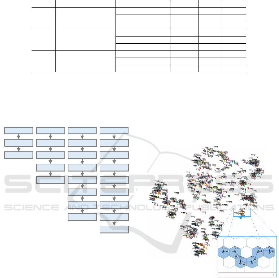
Table 1: Subsets range and users subset datasets deﬁned.

Subset #UCells subset range User subset dataset #UCells #Cells #Paths

700-1299

726 34645 34641

917 35604 35600

1192 61833 61829

1300-2449

1331 48099 48094

1758 27624 27620

2415 43418 43414

2500-3700

2488 67895 67891

3502 48499 48494

3638 64303 64299

current Neural Network (SRNN), Simple Gate Recur-

rent Unit (SGRU), Stacked Long Short-Term Mem-

ory (SLSTM), and Convolutional Long Short-Term

Memory (CLSTM).

RNN

Softmax Dropout

Flatten

Softmax

GRU LSTM Conv1D

MaxPooling1D

Dropout Dropout

LSTM

Dropout LSTM

DropoutTimeDistributed

TimeDistributedFlatten

FlattenSoftmax

Softmax

SRNN SGRU SLSTM CLSTM

Embedding Embedding Embedding Embedding

Figure 3: ML architectures.

These ML architectures were trained with and

without W2V pre-trained weights in a classiﬁcation

problem to predict the user mobility, and training time

was compared. To produce a distributed representa-

tion of words in W2V two models are available: Con-

tinuous Bag-Of-Words (CBOW) or Skip Gram. The

difference between both is that with CBOW a group

of context words is used to predict the target word

and with Skip Gram, given a target word, the context

words are predicted. By analogy #Cells represents the

number of words and #UCells the number of unique

words in each user subset dataset representing a tra-

jectory. After pre-processing the trajectory for each

user, W2V creates a cell ID embeddings using Skip

Gram architecture, resulting in a vector space where

cell IDs that are neighbours are close to each other

in the space. Fig. 4 presents the lower dimensional

space with the cell IDs from 18 months of trajec-

tories carried by user U

that are plotted with 726

unique cell IDs. As word embedding is hard to vi-

sualize (Molino et al., 2019), t-distributed Stochastic

Neighbor Embedding (T-SNE) tool (Van Der Maaten

and Hinton, 2008) was used to plot the high dimen-

sional data using a dimension reduction while keeping

the relative pairwise similarities of the corresponding

low-dimensional points in the embedding.

Figure 4: Global neighboring relation between cell IDs and

user path example.

The experiments were performed using a work-

station with 32GB of RAM memory, featuring an In-

tel I7 quad core processor and a GPU Nvidia Quadro

M1200 with 4GB of RAM. As ML platform, Ana-

conda (Anaconda Software Distribution, 2020) with

Keras (Chollet et al., 2015) & TensorFlow 2.0 (Abadi

et al., 2015) was used.

Fig. 5 presents the four Neural Network (NN)

models that were tested using the ML architectures

deﬁned in Fig. 3, i.e.:

• SRNN versus SRNN+W2V

DeLTA 2021 - 2nd International Conference on Deep Learning Theory and Applications

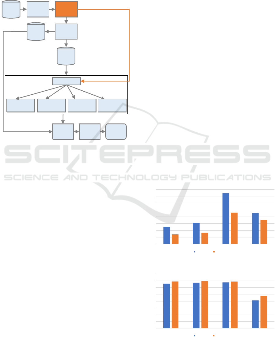
• SGRU versus SGRU+W2V

• SLSTM versus SLSTM+W2V

• CLSTM versus CLSTM+W2V

Features

Extration

MDC

Dataset

Word2Vec

Encoded

Cell ID

Sequences

Train

Dataset

Evaluation Model Prediction

Embedding

SRNN

SRNN+W2V

SGRU

SGRU+W2V

SLSTM

SLSTM+W2V

CLSTM

CLSTM+W2V

Test

Dataset

Pre-Trained

Weights

Figure 5: ML architectures.

Features were extracted from each subset dataset

and paths prepared to be used as input sentences in

W2V. Then encoded cell IDs sentences were divided

into two datasets with 75% to be used in the training

process and 25% to test the training process. All ar-

chitectures were conﬁgured to use softmax function

to normalize the output of the NN to a probability

distribution over the unique cells in each trajectory

that are the predicted output labels. To stop the train-

ing once the model performance is not improving,

EarlyStopping was activated with a patience value of

100 epochs and mindelta of 0.001% in validation ac-

curacy, i.e., if there is no improvement in the last 100

epochs, training will be stopped. In each train, time

counter was started just before the model training and

stopped after the model ﬁt, training time from each

test were kept for further analysis.

4 RESULTS AND ANALYSIS

Results were divided in 2 tables: Table 2 presents the

results from simple models (SRNN, SGRU) and Ta-

ble 3 presents the results from more complex models

(SLSTM, CLSTM). In both Tables the data has been

upwardly ordered by #UCells per user subset dataset

and, for each test, the number of epochs, training time

(TT) in seconds and validation accuracy (ValAcc) in

percentage are shown. Table 4 compiles the aver-

age results obtained in the 4 tested architectures and

presents the differences with regard to the use of W2V

in terms of number of epochs, training time (TT) in

seconds and validation accuracy (ValAcc) in percent-

age.

The results presented in Table 2 and Table 3 show

a trend where datasets with lower #UCells values re-

sult in a shorter training time and higher validation

accuracy, this is due to the fact of the computational

cost of training a multilabel classiﬁer may be strongly

affected by the number of labels.

As seen in Table 4 architectures SRNN+W2V,

SGRU+W2V, SLSTM+W2V, CLSTM+W2V have

improved in terms of lower training time and higher

validation accuracy. The training time reduction ra-

tio is in architecture SRNN+W2V from 32% to 54%

(43% in average), in SGRU+W2V from 10% to 57%

(43% in average), in SLSTM+W2V from 16% to 49%

(33% in average) and in CLSTM+W2V from 8% to

41% (22% in average). Globally comparing the ar-

chitectures, the training time reduction ratio is in av-

erage 36%. In terms of validation accuracy there is

also an improvement: in SRNN+W2V from 1 per-

centage point (pp) to 6 pps (3 pps in average), in

SGRU+W2V from 0 pp to 4 pps (2 pps in average),

in SLSTM+W2V from 1 pp to 2 pps (1 pp in aver-

age) and in CLSTM+W2V from 2 pps to 12 pps (7

pps in average), globally architectures improved the

validation accuracy in average by 3 pps.

2536

3085

7450

4547

1410

1644

4596

3523

1000

2000

3000

4000

5000

6000

7000

8000

SRNN SGRU SLSTM CLSTM

Training Time (s)

Without W2V With W2V

Figure 6: Average training time per architecture.

66%

67%

68%

41%

69%

48%

10%

20%

30%

40%

50%

60%

70%

80%

SRNN SGRU SLSTM CLSTM

Validation Accuracy (%)

Without W2V With W2V

Figure 7: Average validation accuracy per architecture.

Using Syntactic Similarity to Shorten the Training Time of Deep Learning Models using Time Series Datasets: A Case Study

Table 2: Architectures SRNN and SGRU training-related metric comparison without and with W2V.

Users

SRNN SRNN+W2V vs SRNN SGRU SGRU+W2V vs SGRU

Epoch

(s)

ValAcc

(%)

Epoch

(s)(%)

ValAcc

(p.p.)

Epoch

(s)

ValAcc

(%)

Epoch

(s)(%)

ValAcc

(p.p.)

419 1262 77% -176 -529 -42% +1 595 1751 78% -55 -177 -10% +1

538 1715 78% -209 -682 -40% +2 643 1995 78% -323 -1007 -50% +2

444 2430 71% -206 -1117 -46% +1 683 3568 72% -364 -1775 -50% 0

503 2195 65% -164 -693 -32% +3 618 2725 66% -245 -1117 -41% +2

625 1598 73% -272 -690 -43% +3 658 1777 73% -229 -615 -35% +3

756 3152 61% -346 -1441 -46% +6 657 3004 63% -356 -1626 -54% +4

552 3501 57% -272 -1728 -49% +4 660 4546 60% -373 -2581 -57% +2

742 3607 54% -400 -1944 -54% +5 599 3305 56% -213 -1165 -35% +3

522 3363 57% -200 -1306 -39% +4 688 5094 58% -391 -2905 -57% +4

Avg 567 2536 66% -249 -1126 -43% +3 645 3085 67% -283 -1441 -43% +2

Table 3: Architectures SLSTM and CLSTM training-related metric comparison without and with W2V.

Users

SLSTM SLSTM+W2V vs SLSTM CLSTM CLSTM+W2V vs CLSTM

Epoch

(s)

ValAcc

(%)

Epoch

(s)(%)

ValAcc

(p.p.)

Epoch

(s)

ValAcc

(%)

Epoch

(s)(%)

ValAcc

(p.p.)

619 2844 79% -169 -780 -27% +1 738 2497 47% -202 -671 -27% +3

579 3113 78% -147 -785 -25% +1 637 2321 45% -164 -613 -26% +3

402 4272 72% -65 -687 -16% +2 641 4076 45% -260 -1668 -41% +2

413 3628 67% -106 -921 -25% +1 624 3200 43% -51 -264 -8% +5

717 4684 74% -301 -1960 -42% +1 799 2625 41% -69 -229 -9% +12

417 6198 65% -138 -2042 -33% +1 698 4371 38% -172 -1085 -25% +8

451 10695 60% -199 -4700 -44% +1 651 6451 38% -120 -1205 -19% +8

456 14289 56% -203 -6983 -49% +2 789 7433 35% -182 -1737 -23% +11

429 17328 58% -170 -6825 -39% +1 617 7949 39% -136 -1741 -22% +8

Avg 498 7450 68% -166 -2854 -33% +1 688 4547 41% -151 -1024 -22% +7

Table 4: Global architectures average comparison - number of epochs (Epoch), training time (TT) and validation accuracy

(ValAcc).

Arch.

Without W2V With W2V

Differences

Epoch

(s)

ValAcc

(%)

Epoch

(s)

ValAcc

(%)

Epoch

(s)(%)

ValAcc

(p.p.)

SRNN 567 2536 66% 317 1410 69% -249 -1126 -43% +3

SGRU 645 3085 67% 361 1644 69% -283 -1441 -43% +2

SLSTM 498 7450 68% 332 4596 69% -166 -2854 -33% +1

CLSTM 688 4547 41% 538 3523 48% -151 -1024 -22% +7

Avg. 599 4405 60% 387 2794 64% -212 -1611 -36% +3

43%

33%

22%

10%

15%

20%

25%

30%

35%

40%

45%

50%

SRNN SGRU SLSTM CLSTM

Training Time Reduction Ratio (%)

Architectures

Figure 8: Training time reduction ratio.

Fig. 6 shows the average training time in seconds

per architecture, it is stated that simple architectures

needed less time to train each dataset and that the use

of W2V reduced the training time.

Fig. 7 shows the average validation accuracy per

architecture. SRNN, SGRU, SLSTM obtained better

validation accuracy than CLSTM, the validation accu-

racy is higher when W2V is integrated by each archi-

tecture and CLSTM takes better advantage of using

W2V.

Fig 8 shows the training time reduction ratio ob-

tained by the usage of W2V which is positive in the

4 architectures and being more signiﬁcant in simple

architectures.

Analyzing the global average values, it can be

concluded that in less complex architectures, such as

SRNN+W2V and SGRU+W2V, better results are ob-

tained both in training time and accuracy. In terms of

validation accuracy SRNN+W2V and SGRU+W2V

obtained the same values than SLSTM+W2V but in

average improvements obtained in training time are

10% higher. Comparing training time and validation

accuracy from architecture CLSTM+W2V, the gain is

lower in terms of training time (less 22% in average)

but although the validation accuracy is low, the gains

are 7 pps higher than CLSTM.

DeLTA 2021 - 2nd International Conference on Deep Learning Theory and Applications

5 CONCLUSIONS

When building and deploying a ML model, the train-

ing stage one is the most time-consuming. In order to

reduce the training time of models using time series

datasets, syntactic similarity can be used.

In order to test this assumption, this paper de-

signed a case study based on MNOs scenario used to

predict client mobility. In this case study, a set of ML

models, namely RNN, GRU, LSTM and CNN, were

tested with the integration of the W2V to reduce the

training time.

The experimental results show that as the num-

ber of labels that can be predicted increases, the train-

ing time also increases. When comparing the results

obtained for different architectures, the use of pre-

trained weights from W2V presented a training time

reduction ratio between 22% and 43% and improved

the validation accuracy between 1 pp and 7 pps result-

ing in an overall gain of 3 pps.

These results show that the integration of W2V

pre-trained weights at the initial training stage may

reduce the ML training time in other scenarios such

as forecasting mobility in networks, epidemic control,

transportation management, urban planning, location-

based services, or management of cellular network re-

sources.

REFERENCES

Abadi, M., Agarwal, A., Barham, P., Brevdo, E., Chen,

Z., Citro, C., Corrado, G. S., Davis, A., Dean, J.,

Devin, M., Ghemawat, S., Goodfellow, I., Harp, A.,

Irving, G., Isard, M., Jia, Y., Jozefowicz, R., Kaiser,

L., Kudlur, M., Levenberg, J., Man

e, D., Monga, R.,

Moore, S., Murray, D., Olah, C., Schuster, M., Shlens,

J., Steiner, B., Sutskever, I., Talwar, K., Tucker, P.,

Vanhoucke, V., Vasudevan, V., Vi

egas, F., Vinyals,

O., Warden, P., Wattenberg, M., Wicke, M., Yu, Y.,

and Zheng, X. (2015). TensorFlow: Large-scale ma-

chine learning on heterogeneous systems. Web site.

Software available from tensorﬂow.org (accessed on 1

February 2021).

Anaconda Software Distribution (2020). Anaconda soft-

ware distribution. Web site. Software available from

https://www.anaconda.com (accessed on 1 February

2021).

Chollet, F. et al. (2015). Keras. Web site. Software avail-

able from https://github.com/fchollet/keras (accesse-

don1 February 2021).

Collobert, R., Farabet, C., and Kavukcuo

glu, K. (2008).

Torch — Scientiﬁc computing for LuaJIT. NIPS Work-

shop on Machine Learning Open Source Software.

Fan, X., Guo, L., Han, N., Wang, Y., Shi, J., and Yuan,

Y. (2018). A Deep Learning Approach for Next Lo-

cation Prediction. Proceedings of the 2018 IEEE

22nd International Conference on Computer Sup-

ported Cooperative Work in Design, CSCWD 2018,

(May 2018):630–635.

Gonz

alez, M. C., Hidalgo, C. A., and Barab

asi, A. L.

(2008). Understanding individual human mobility

patterns. Nature, 453(7196):779–782.

Hashimoto, K., Stenetorp, P., Miwa, M., and Tsuruoka, Y.

(2015). Task-oriented learning of word embeddings

for semantic relation classiﬁcation. CoNLL 2015 -

19th Conference on Computational Natural Language

Learning, Proceedings, pages 268–278.

Jeung, H., Lu, H., Sathe, S., and Yiu, M. L. (2014). Manag-

ing evolving uncertainty in trajectory databases. IEEE

Transactions on Knowledge and Data Engineering,

26(7):1692–1705.

Jia, Y., Shelhamer, E., Donahue, J., Karayev, S., Long, J.,

Girshick, R., Guadarrama, S., and Darrell, T. (2014).

Caffe: Convolutional architecture for fast feature em-

bedding. arXiv preprint arXiv:1408.5093.

Kim, Y. (2014). Convolutional neural networks for sentence

classiﬁcation. EMNLP 2014 - 2014 Conference on

Empirical Methods in Natural Language Processing,

Proceedings of the Conference, pages 1746–1751.

Kiukkonen, N., Blom, J., Dousse, O., Gatica-perez, D.,

and Laurila, J. (2010). Towards rich mobile phone

datasets: Lausanne data collection campaign.

Kotz, D., Henderson, T., and McDonald, C. (2005). Craw-

dad archive: a community resource for archiving wire-

less data at dartmouth. Web site. Archive available

from https://www.crawdad.org (accessed on 1 Febru-

ary 2021).

Kretowicz, W. and Biecek, P. (2020). MementoML: Perfor-

mance of selected machine learning algorithm conﬁg-

urations on OpenML100 datasets. pages 1–7.

Laurila, J. K., Gatica-Perez, D., Aad, I., Blom, J., Bornet,

O., Do, T. M. T., Dousse, O., Eberle, J., and Miettinen,

M. (2013). From big smartphone data to worldwide

research: The Mobile Data Challenge. Pervasive and

Mobile Computing, 9(6):752–771.

Microsoft Azure (2017). The Microsoft Cogni-

tive Toolkit - Cognitive Toolkit - CNTK —

Microsoft Docs. Software available from

https://github.com/Microsoft/CNTK (accessed on

1 February 2021).

Mikolov, T., Chen, K., Corrado, G., and Dean, J. (2013).

Efﬁcient estimation of word representations in vector

space. 1st International Conference on Learning Rep-

resentations, ICLR 2013 - Workshop Track Proceed-

ings, pages 1–12.

Miranda, C. S. and Von Zuben, F. J. (2015). Reducing the

Training Time of Neural Networks by Partitioning.

Molino, P., Wang, Y., and Zhang, J. (2019). Parallax: Vi-

sualizing and understanding the semantics of embed-

ding spaces via algebraic formulae. ACL 2019 - 57th

Annual Meeting of the Association for Computational

Linguistics, Proceedings of System Demonstrations,

pages 165–180.

Reif, M., Shafait, F., and Dengel, A. (2011). Prediction of

classiﬁer training time including parameter optimiza-

tion. Lecture Notes in Computer Science (including

Using Syntactic Similarity to Shorten the Training Time of Deep Learning Models using Time Series Datasets: A Case Study

subseries Lecture Notes in Artiﬁcial Intelligence and

Lecture Notes in Bioinformatics), 7006 LNAI(June

2014):260–271.

Shi, S., Wang, Q., Xu, P., and Chu, X. (2017). Bench-

marking state-of-the-art deep learning software tools.

Proceedings - 2016 7th International Conference on

Cloud Computing and Big Data, CCBD 2016, pages

99–104.

Tang, D., Qin, B., and Liu, T. (2015). Document model-

ing with gated recurrent neural network for sentiment

classiﬁcation. Conference Proceedings - EMNLP

2015: Conference on Empirical Methods in Natural

Language Processing, (September):1422–1432.

Van Der Maaten, L. and Hinton, G. (2008). Visualizing

Data using t-SNE. Technical report.

Wang, C., Zhao, Z., Sun, Q., and Zhang, H. (2018). Deep

Learning-based Intelligent Dual Connectivity for Mo-

bility Management in Dense Network. pages 1–5.

Wickramasuriya, D. S., Perumalla, C. A., Davaslioglu, K.,

and Gitlin, R. D. (2017). Base station prediction and

proactive mobility management in virtual cells using

recurrent neural networks. In 2017 IEEE 18th Wire-

less and Microwave Technology Conference, WAMI-

CON 2017, pages 1–6. IEEE.

Yang, C., Sun, M., Zhao, W. X., Liu, Z., and Chang, E. Y.

(2018). A Neural Network Approach to Joint Model-

ing Social Networks and Mobile Trajectories. Techni-

cal report.

Yih, W. T., He, X., and Meek, C. (2014). Semantic pars-

ing for single-relation question answering. 52nd An-

nual Meeting of the Association for Computational

Linguistics, ACL 2014 - Proceedings of the Confer-

ence, 2:643–648.

Zayats, V. and Ostendorf, M. (2018). Conversation Mod-

eling on Reddit Using a Graph-Structured LSTM.

Transactions of the Association for Computational

Linguistics, 6:121–132.

Zheng, Y., Fu, H., Xie, X., Ma, W.-Y., and Li,

Q. (2011). Geolife GPS trajectory dataset -

User Guide, geolife gps trajectories 1.1 edition.

Download available at https://www.microsoft.com/en-

us/download/details.aspx?id=52367 (accessed on 1

February 2021).

DeLTA 2021 - 2nd International Conference on Deep Learning Theory and Applications

100