
Learning-based Optimal Control of Constrained Switched Linear
Systems using Neural Networks
Lukas Markolf
a
and Olaf Stursberg
b
Control and System Theory, Dept. of Electrical Engineering and Computer Science, University of Kassel,
Wilhelmsh
¨
oher Allee 73, 34121 Kassel, Germany
Keywords:
Neural Networks, Intelligent Control, Hybrid Systems, Approximate Dynamic Programming.
Abstract:
This work considers (deep) artificial feed-forward neural networks as parametric approximators in optimal
control of discrete-time switched linear systems with controlled switching. The proposed approach is based on
approximate dynamic programming and allows the fast computation of (sub-)optimal discrete and continuous
control inputs, either by approximating the optimal cost-to-go functions or by approximating the optimal
discrete and continuous input policies. An important property of the approach is the satisfaction of polytopic
state and input constraints, which is crucial for ensuring safety, as required in many control applications. A
numeric example is provided for illustration and evaluation of the approaches.
1 INTRODUCTION
In many applications, continuous and discrete con-
trols coexist as, e.g., in all production or processing
systems which are equipped with continuous feed-
back controllers and supervisory controllers. Typi-
cally, the two types of controllers are considered and
designed separately, not only to split the correspond-
ing functions, but also to simplify the design task. The
separate design, however, may lead to degraded per-
formance if the two parts lead to opposing effects on
the plant at the same time. This motivates to investi-
gate techniques that optimize continuous and discrete
controls simultaneously. This paper considers the de-
sign of optimizing feedback controllers for discrete-
time switched linear systems (SLS). Such systems,
which constitute a special class of hybrid systems
(Branicky et al., 1998), allow to switch between lin-
ear dynamics by use of the discrete controls. Note
that this externally triggered switching is different
from the class of discrete-time piecewise affine sys-
tems (Sontag, 1981), in which switching occurs au-
tonomously and is bound to the fact that the continu-
ous state enters a new (polytopic) state region.
If optimization-based computation of control
strategies for SLS is considered, typically mixed-
integer programming problems are encountered,
which are known to be NP hard problems, see e.g.
a
https://orcid.org/0000-0003-4910-8218
b
https://orcid.org/0000-0002-9600-457X
(Bussieck and Pruessner, 2003). Nevertheless, for the
optimal open-loop control of discrete-time SLS with
quadratic performance measure and without state and
input constraints relatively efficient techniques have
been proposed, see e.g. in (G
¨
orges et al., 2011). The
complexity there is reduced via pruning of the search
tree and accepting sub-optimal solutions. An on-line
open-loop control approach for the case with state
and input constraints is described in (Liu and Sturs-
berg, 2018), where a trade-off between performance
and applicability is obtained by tree search with cost
bounds and search heuristics.
In contrast, the present paper aims at determining
optimal closed-loop control laws to select the con-
tinuous and discrete inputs for any state of the SLS.
In principle, this task can be solved by dynamic pro-
gramming (Bellman, 2010), but the complexity pre-
vents the use for most systems. The concept of ap-
proximate dynamic programming (ADP) (Bertsekas,
2019) is more promising in this respect, but has not
yet been used for controller synthesis of SLS with
consideration of constraints – this is the very objec-
tive of this paper. The approach is to learn the control
law from a dataset, which may originate from off-line
solution of mixed-integer programming problems for
selected initial states, or from approximate dynamic
programming over short horizons. The use of (deep)
neural networks (NN) are proposed as parametric ar-
chitectures for either approximating cost-to-go func-
tions, or the continuous-discrete control laws. NN as
90
Markolf, L. and Stursberg, O.
Learning-based Optimal Control of Constrained Switched Linear Systems using Neural Networks.
DOI: 10.5220/0010581600900098
In Proceedings of the 18th Inter national Conference on Informatics in Control, Automation and Robotics (ICINCO 2021), pages 90-98
ISBN: 978-989-758-522-7
Copyright
c
2021 by SCITEPRESS – Science and Technology Publications, Lda. All rights reserved

parametric approximators are appealing due to their
property of universal approximation (Cybenko, 1989;
Hornik et al., 1989) and the recent success of deep
learning (Goodfellow et al., 2016). For the different
task of model predictive control of purely continuous-
valued systems, recent work has shown that the use
of NN (determined off-line) can lead to solutions of
problems in which full on-line computation takes pro-
hibitively long, see e.g. (Chen et al., 2018; Hertneck
et al., 2018; Karg and Lucia, 2020; Paulson and Mes-
bah, 2020; Markolf and Stursberg, 2021). This mo-
tivates for the present paper to train NN also for op-
timal control of SLS, despite the complexity arising
from the mixed inputs. While the analysis of neu-
ral networks is known to be challenging due to their
nonlinear and often large-scale structure, this paper
makes use of the methods developed in (Chen et al.,
2018) and (Markolf and Stursberg, 2021) to ensure
the satisfaction of state and input constraints in addi-
tion.
The considered problem is stated in Sec. 2, while
Sec. 3 shows how an ADP approach can be formu-
lated for SLS in principle. The specific choice of NN
as function approximators and solutions for consider-
ing the constraints, as well as the main algorithms are
detailed in Sec. 4. A numerical example is provided
in Sec. 5, before the paper is concluded in Sec. 6.
2 PROBLEM STATEMENT
This paper considers discrete-time and constrained
switched systems of the form:
x
k+1
= f
v
k
(x
k
,u
k
), k ∈ {0,..., N − 1}, (1)
where k is the time index, N a finite time horizon,
x
k
∈ R
n
x
the continuous state vector, u
k
∈ R
n
u
the
vector of continuous control inputs, and v
k
∈ V =
{v
[1]
,.. .,v
[n
v
]
} the discrete control input determining
the subsystem f
v
k
: R
n
x
× R
n
u
→ R
n
x
selected at time
k. The focus in this paper is on switched linear sys-
tems with matrices A
v
k
and B
v
k
of appropriate dimen-
sions:
f
v
k
(x
k
,u
k
) = A
v
k
x
k
+ B
v
k
u
k
, k ∈ {0,. ..,N − 1}.
(2)
The states and inputs are constrained to polytopes X
and U:
x
k
∈ X =
x ∈ R
n
x
|H
X
x ≤ h
X
, (3)
u
k
∈ U =
u ∈ R
n
u
|H
U
u ≤ h
U
, (4)
with matrices H
X
,H
U
, and vectors h
X
,h
U
. For a
given state x
k
, k ∈ {0,. .., N − 1} and input sequences
over a time span {k,. .., N − 1}:
φ
u
k
:= {u
k
,.. .,u
N−1
}, (5)
φ
v
k
:= {v
k
,.. .,v
N−1
}, (6)
the corresponding unique state sequence is denoted
by:
φ
x
k
:= {x
k
,.. .,x
N
} (7)
and obtained from (1).
Let X
N
⊆ X be a target set specified as polytope:
X
N
=
x ∈ R
n
x
|H
X
N
x ≤ h
X
N
⊆ X. (8)
Furthermore, let a sequence of state sets
{X
0
,.. .,X
N−1
} be defined, satisfying:
X
k
= {x ∈ X |for each v ∈ V : ∃u ∈ U such that
f
v
(x,u) ∈ X
k+1
}, k ∈ {0,. ..,N − 1},
(9)
i.e., for any state x
k
∈ X
k
, k ∈ {0,. .., N − 1} and
an arbitrary choice of the discrete input v
k
∈ V , at
least one admissible continuous input u
k
∈ U exists
such that f
v
k
(x
k
,u
k
) ∈ X
k+1
. The actual computation
of these sets will be addressed later in Sec. 4.
The following fact then obviously holds:
Proposition 1. If X
0
is nonempty, then for each ini-
tialization x
0
∈ X
0
and each discrete input sequence
φ
v
0
at least one admissible continuous input sequence
φ
u
0
exists that transfers x
0
into the target set X
N
,
while satisfying x
i
∈ X
i
, i ∈ {0,... ,N} and u
i
∈ U,
i ∈ {0, ... ,N − 1}.
For introducing costs, assume that φ
x
k
has been de-
termined for a given state x
k
at time k ∈ {0, ..., N −
1}, and for given input sequences φ
u
k
and φ
v
k
. Then let
J
k
(φ
x
k
,φ
u
k
,φ
v
k
) denote the total cost associated with this
evolution:
J
k
(φ
x
k
,φ
u
k
,φ
v
k
) = g
N
(x
N
) +
N−1
∑
i=k
g
i,v
i
(x
i
,u
i
),
(10)
where g
N
: X → R
≥0
denotes a terminal cost, and
g
k,v
k
: X × U → R
≥0
, k ∈ {0,.. .,N − 1} a stage cost
for v
k
∈ V at stage k. Furthermore, let J
∗
k
(x) be
the optimal cost-to-go for steering a state x at time
k ∈ {0,. . .,N − 1} into the target set X
N
within N − k
steps, while satisfying x
i
∈ X
i
, i ∈ {k,... ,N} and
u
i
∈ U, i ∈ {k,..., N − 1}, i.e.:
J
∗
k
(x) = min
φ
u
k
,φ
v
k
J
k
(φ
x
k
,φ
u
k
,φ
v
k
) (11a)
subject to:
x
k
= x, (11b)
x
i+1
= A
v
i
x
i
+ B
v
i
u
i
, i ∈ {k,... ,N − 1}, (11c)
u
i
∈ U, i ∈ {k, ... ,N − 1}, (11d)
x
i
∈ X
i
, i ∈ {k,... ,N}. (11e)
Learning-based Optimal Control of Constrained Switched Linear Systems using Neural Networks
91

By convention, J
∗
k
is set to infinity for the case that
(11) is infeasible for a specific state x ∈ R
n
x
. Subse-
quently, the constraints (11d) and (11e) are replaced
by u
i
∈ U
i
(x
i
,v
i
), i ∈ {k , ... ,N − 1}. Here, U
k
(x
k
,v
k
),
k ∈ {0,. .., N − 1} denotes a set that depends on
the state x
k
∈ X and the discrete input v
k
∈ V , and
contains all the continuous inputs u
k
∈ U for which
f
v
k
(x
k
,u
k
) ∈ X
k+1
:
U
k
(x,v) = {u ∈ U | f
v
(x,u) ∈ X
k+1
}. (12)
Again, the actual computation of these sets will be
addressed later in Sec. 4
The following problem is considered in this work:
Problem 1 (Finite-Horizon Control Problem). Find
an optimal control law which assigns to each state
x
k
∈ X
k
at time instant k ∈ {0,.. .,N − 1} a pair of
optimal admissible inputs v
∗
k
∈ V and u
∗
k
∈ U
k
(x
k
,v
∗
k
),
such that for any x
0
∈ X
0
, the cost J
0
φ
x
∗
0
,φ
u
∗
0
,φ
v
∗
0
obtained for the resulting sequences φ
x
∗
0
, φ
u
∗
0
, φ
v
∗
0
is
optimal, i.e.: J
0
φ
x
∗
0
,φ
u
∗
0
,φ
v
∗
0
= J
∗
0
(x
0
).
In order to allow for the use of gradient methods
to tackle this problem, as proposed in (Markolf and
Stursberg, 2021), the following assumption is made,
which is not practically restrictive.
Assumption 1. Suppose that the functions g
k,v
(x,u),
k ∈ {0,. .., N − 1}, v ∈ V in (10) are continuously dif-
ferentiable with respect to u ∈ U.
3 APPROXIMATE DYNAMIC
PROGRAMMING FOR SLS
In theory, dynamic programming (DP) provides a
scheme to solve the Problem 1: Starting from:
J
∗
N
(x
N
) := g
N
(x
N
), (13)
the DP algorithm proceeds backward in time from
N − 1 to 0 to compute the optimal cost-to-go func-
tions:
J
∗
k
(x
k
) = min
v
k
∈V
u
k
∈U
k
(x
k
,v
k
)
h
g
k,v
k
(x
k
,u
k
) + J
∗
k+1
( f
v
k
(x
k
,u
k
))
i
.
(14)
Such a version of the DP-algorithm is similar to the
standard one without discrete inputs, as can be found
e.g. in (Bertsekas, 2005). Provided that the opti-
mal cost-to-go values J
∗
k
are known for all relevant
x
k
and k, the optimal discrete and continuous input
sequences φ
v
∗
0
and φ
u
∗
0
for x
0
∈ X
0
can be constructed
in a forward manner by:
(v
∗
k
,u
∗
k
) ∈arg min
v
k
∈V
u
k
∈U
k
(x
∗
k
,v
k
)
h
g
k,v
k
(x
∗
k
,u
k
) + J
∗
k+1
f
v
k
(x
∗
k
,u
k
)
i
,
(15)
with x
∗
0
= x
0
and x
∗
k+1
= f
v
∗
k
(x
∗
k
,u
∗
k
).
For the general setup considered in this work, the
DP algorithm does not lead to closed-form expres-
sions for J
∗
k
and for the respective optimal policies
denoted by:
π
u
∗
:= {µ
u
∗
0
(·),.. .,µ
u
∗
N−1
(·)}, µ
u
∗
k
: X → U, (16)
π
v
∗
:= {µ
v
∗
0
(·),.. .,µ
v
∗
N−1
(·)}, µ
v
∗
k
: X → V. (17)
Hence, numeric solution is necessary, but is known
to suffer from the curse of dimensions, thus limiting
practical applicability.
However, the optimal cost-to-go functions J
∗
k
can
be approximated by parametric functions
˜
J
k
with real-
valued parameter vectors r
J
k
, constituting a so-called
approximation in value space (Bertsekas, 2019). The
prediction of the optimal cost-to-go J
∗
k
by
˜
J
k
given
some state x
k
is a typical regression task. Suppose for
a moment that a parametric function
˜
J
k
and a data set
consisting of state-cost pairs (x
s
k
,J
s
k
), s ∈ {1, ... ,q
J
k
}
are available, where each J
s
k
is a regression target pro-
viding the desired value for the corresponding exam-
ple state x
s
k
. On this basis, the parameter vector r
J
k
of the parametric function
˜
J
k
can be adapted with the
objective to improve the performance on the consid-
ered regression task by learning from the data set.
The mean squared error is here (as usual) consid-
ered as performance measure. Such an adaption pro-
cedure for r
J
k
, typically called training, is an exam-
ple for supervised learning. A challenge hereby is to
perform also well on previously not explored states
x
k
, which distinguishes the training procedure from
pure optimization. For a more detailed treatment, see
e.g. (Goodfellow et al., 2016).
The following Algorithm 1, which extends the se-
quential DP procedure from (Bertsekas, 2019) to SLS,
provides an approach for training the parametric ap-
proximators
˜
J
k
in a recursive manner (similar to the
typical DP procedure). Once the parametric approx-
imators
˜
J
k
are trained, approximations of the optimal
discrete and continuous input sequences, denoted as
φ
˜v
0
and φ
˜u
0
, can be constructed for x
0
∈ X
0
in a forward
manner, similar to (15):
( ˜v
k
, ˜u
k
) ∈arg min
v
k
∈V
u
k
∈U
k
( ˜x
k
,v
k
)
h
g
k,v
k
( ˜x
k
,u
k
) +
˜
J
k+1
f
v
k
( ˜x
k
,u
k
),r
J
k+1
i
,
(18)
ICINCO 2021 - 18th International Conference on Informatics in Control, Automation and Robotics
92
with ˜x
0
= x
0
and ˜x
k+1
= f
˜v
k
( ˜x
k
, ˜u
k
).
Another way to obtain approximations of the op-
timal discrete and continuous input sequences is the
approximation of the optimal policies π
v
∗
and π
u
∗
by
so-called parametric policies:
π
˜v
= {µ
˜v
1
(·,r
v
1
),.. .,µ
˜v
N−1
(·,r
v
N−1
)},
with µ
˜v
k
(·,r
v
k
) : X → V, (19)
π
˜u
= {µ
˜u
1
(·,r
u
1
),.. .,µ
˜u
N−1
(·,r
u
N−1
)},
with µ
˜u
k
(·,r
u
k
) : X → U
k
(·,µ
˜v
k
(·,r
v
k
)). (20)
This approach is an example of an approximation in
policy space (Bertsekas, 2019). Again, the parame-
ter vectors r
u
k
and r
v
k
can be adapted by standard su-
pervised learning techniques on the basis of avail-
able data sets (x
s
k
,u
s
k
), s ∈ {1,. .., q
u
k
} and (x
s
k
,v
s
k
),
s ∈ {1,.. .,q
v
k
}, respectively. The data may originate
from solutions of (18), constituting an example of ap-
proximation in policy space on top of approximation
in value space.
4 OPTIMAL CONTROL OF SLS
WITH CONSTRAINTS USING
NN
Based on the rather conceptual derivations in the pre-
ceding chapter, the specific approach for synthesiz-
ing optimal control laws based on NN for SLS with
input and state constraints is now described. Two
procedures of using (deep) neural networks as para-
metric architectures for the approximation of the op-
timal continuous and discrete input sequences are pro-
posed, one by approximation in value space, and the
other by approximation in policy space. In both cases,
Algorithm 1: Sequential Dynamic Programming.
1:
˜
J
N
(x
N
,r
J
N
) := g
N
(x
N
)
2: for k = N − 1 to 0 do
3: Generate a large number of states x
s
k
, s ∈
{1,.. .,q
J
k
} by sampling the state space X
k
4: for s = 1 to q
J
k
do
5:
J
s
k
= min
v∈V
u∈U
k
(
x
s
k
,v
)
h
g
k,v
(x
s
k
,u) +
˜
J
k+1
f
v
(x
s
k
,u), r
J
k+1
i
6: end for
7: Determine r
J
k
by training with (x
s
k
,J
s
k
), s ∈
{1,.. .,q
J
k
}
8: end for
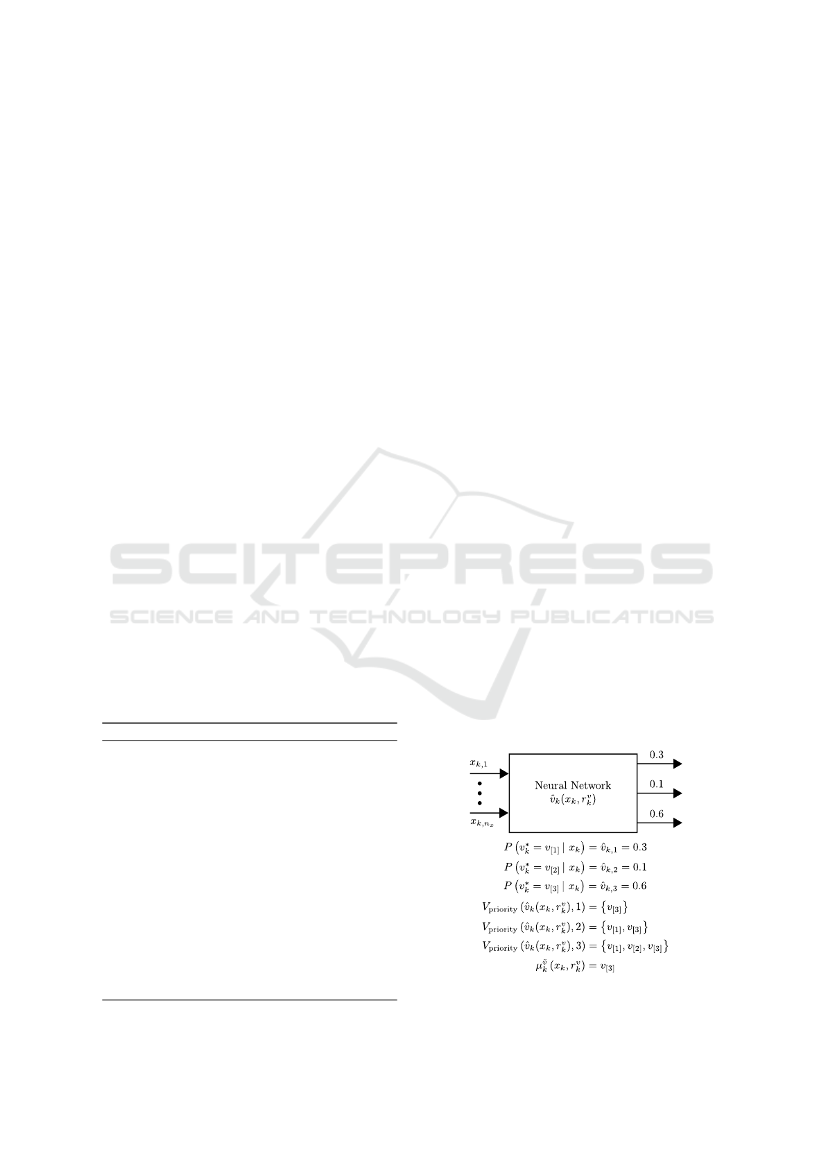
neural networks ˆv
k
, k ∈ {0, ... ,N − 1} with softmax
output units and parameter vectors r
v
k
are employed
to obtain for each x
k
∈ X
k
an n
v
-dimensional output
vector with ˆv
k,i
(x
k
,r
v
k
) = P(v
∗
k
= v
[i]
|x
k
). Thus, the
outputs of the neural network ˆv
k
determine for x
k
a
probability distribution over the discrete control in-
puts, where ˆv
k,i
(x
k
,r
v
k
) denotes the probability that the
discrete control input v
[i]
is optimal for x
k
at stage k.
4.1 Approximation in Value Space
Neural networks with continuous and continuously
differentiable activation functions are proposed as
parametric approximators
˜
J
k
for the optimal cost-to-
go functions J
∗
k
, k ∈ {0, ..., N −1}. Furthermore, a set
V
priority
( ˆv
k
,n
priority
) ⊆ V is introduced, which is used
in approximating the optimal discrete and optimal in-
put sequences in a forward manner for given x
0
∈ X
0
and n
priority
∈ {1,. .., n
v
}:
( ˜v
k
, ˜u
k
) ∈arg min
v
k
∈V
priority
(
ˆv
k
(
˜x
k
,r
v
k
)
,n
priority
)
u
k
∈U
k
( ˜x
k
,v
k
)
h
g
k,v
k
( ˜x
k
,u
k
) +
˜
J
k+1
f
v
k
( ˜x
k
,u
k
),r
J
k+1
i
,
(21)
with ˜x
0
= x
0
and ˜x
k+1
= f
˜v
k
( ˜x
k
, ˜u
k
). Here, n
priority
∈
{1,.. .,n
v
} is a user-defined number used to specify
the number of elements in V
priority
( ˆv
k
,n
priority
), where
these elements are selected to be the discrete inputs
with the highest probabilities according to ˆv
k
. This
allows to establish a trade-off in (21) between the
consideration of only a single discrete input (with the
highest probability to be the optimal one) or all dis-
crete inputs contained in V . Fig. 1 provides an exam-
ple of the concept.
It will be addressed in detail in Sec. 4.3 how to
compute U
k
(x,v), k ∈ {0,.. .,N − 1}, and to show that
Figure 1: Example for illustrating the use of the neural net-
work ˆv
k
.
Learning-based Optimal Control of Constrained Switched Linear Systems using Neural Networks
93

U
k
(x,v) in (12) is a polytope for all x ∈ X
k
and v ∈ V .
The architecture of the neural networks and a closed-
form expression for the partial derivative of
˜
J
k
(x,r
J
k
)
with respect to x will be described in Sec. 4.4. The
property that U
k
(x,v), k ∈ {0,. ..,N − 1} is a polytope
and the availability of closed-form expressions for
[∂
˜
J
k
/∂x](x,r
J
k
) open the door for addressing the min-
imization problems in (18), (21), and Algorithm 1 by
applying well-established gradient methods for each
considered discrete input v ∈ V . The satisfaction of
the convex constraints u ∈ U
k
(x,v) in state-of-the-art
methods of this type is not a problem. Hence, the sat-
isfaction of the considered state and input constraints
in (11) is guaranteed, even in case of imperfect ap-
proximations of the optimal cost-to-go functions, or
if the iterative procedure of the gradient method is
stopped before finding a local minimum. This ap-
proach can be based on existing work on gradient-
methods for systems without switching (Markolf and
Stursberg, 2021).
4.2 Approximation in Policy Space
Alternatively, NN can be used directly as parametric
approximators µ
˜u
k
of the optimal continuous policies
µ
u
∗
k
, k ∈ {0,.. .,N − 1}. The optimal discrete input
policies µ
v
∗
k
are approximated by:
µ
˜v
k
(x
k
,r
v
k
) ∈
v
[i]
∈ V |for all j ∈ {1, ... ,n
v
} :
P
v
∗
k
= v
[i]
|x
k
≥ P
v
∗
k
= v
[ j]
|x
k
.
(22)
For a given initial state x
0
∈ X
0
, the scheme is then
to approximate the optimal continuous and discrete
input sequences in forward manner by computing:
˜v
k
= µ
˜v
k
( ˜x
k
,r
v
k
) ∈ V, (23)
˜u
k
= µ
˜u
k
( ˜x
k
, ˜v
k
,r
u
k
) ∈ U
k
( ˜x
k
, ˜v
k
), (24)
with ˜x
0
= x
0
and ˜x
k+1
= f
˜v
k
( ˜x
k
, ˜u
k
).
Provided that µ
˜u
k
(x
k
,v
k
,r
u
k
) ∈ U
k
(x
k
,v
k
) for each
x
k
∈ X
k
and v
k
∈ V , the satisfaction of the state and in-
put constraints considered in (11) is guaranteed. This
can be achieved by projecting the output of the neural
network onto the polytope U
k
(x
k
,v
k
). An approach to
projecting the output of a neural network onto a poly-
tope can be found in (Chen et al., 2018).
4.3 Controllable Sets
For a given v ∈ V , let Pre
v
(X ) be the set of state pre-
decessors to X , i.e. containing all the states x ∈ R
n
x
for which at least one input u ∈ U exists such that
f
v
(x,u) ∈ X :
Pre
v
(X ) = {x ∈ R
n
x
|∃u ∈ U such that f
v
(x,u) ∈ X }.
(25)
If X is a polytope, then Pre
v
(X ) results from a linear
transformation of X , and is thus also a polytope. De-
tails about the computation of Pre
v
(X ) for a polytope
X can be found e.g. in (Borrelli et al., 2017).
Starting from a target set X
N
⊆ X, the sequence of
state sets {X
0
,.. .,X
N−1
} can be computed recursively
as shown in Algorithm 2. Since X
N
is specified in (8)
as polytope, each X
k
, k ∈ {0, ... , N − 1} defined in (9)
is again a polytope:
X
k
=
x ∈ R
n
x
|H
X
k
x ≤ h
X
k
. (26)
For polytopic sets X
k
, k ∈ {0, ... ,N − 1}, also the
sets U
k
(x,v) defined by (12) are polytopes for all x ∈
X
k
and v ∈ V , and given by:
U
k
(x,v) = {u ∈ R
n
u
|H
U
k
(v)u ≤ h
U
k
(x,v)}, (27)
with:
H
U
k
(v) =
H
X
k+1
B
v
H
U
, (28)
h
U
k
(x,v) =
h
X
k+1
− H
X
k+1
A
v
x
h
U
. (29)
4.4 Neural Networks
Feed-forward NN characterized by a chain structure:
h(x) = (h
(L)
◦ ·· · ◦ h
(2)
◦ h
(1)
)(x) (30)
are considered, with final layer h
(L)
and hidden layers
h
(`)
, ` ∈ {1,. .., L−1}. Such structures are commonly
used and detailed information can be found in several
textbooks, see e.g. (Goodfellow et al., 2016). The
output of layer ` is denoted as η
(`)
in the following,
while η
(0)
is defined to be the input of the overall net-
work:
η
(0)
(x) = x, (31)
η
(`)
(x) = (h
(`)
◦ ·· · ◦ h
(1)
)(x). (32)
Here, the hidden layers are (as usual) considered to be
vector-to-vector functions of the form:
h
(`)
(η
(`−1)
) = (φ
(`)
◦ ψ
(`)
)(η
(`−1)
), (33)
with affine and nonlinear transformations ψ
(`)
and
φ
(`)
, respectively. The affine transformation can be
Algorithm 2: Controllable Set Computation.
Input: n
v
, N, X, X
N
Output: X
1
,.. .,X
N−1
1: for k = N − 1 to 0 do
2: X
k
= X
3: for i = 1 to n
v
do
4: X
k
← Pre
v[i]
(X
k+1
) ∩ X
k
5: end for
6: end for
ICINCO 2021 - 18th International Conference on Informatics in Control, Automation and Robotics
94
affected by the choice of the weight matrix W
(`)
and
the bias vector b
(`)
:
ψ
(`)
(η
(`−1)
) = W
(`)
η
(`−1)
+ b
(`)
. (34)
Each layer can be interpreted to consist of parallel act-
ing units, where a positive integer S
(`)
is used here to
describe the number of units in layer `. Each unit i
in layer ` defines a vector-to-scalar function, which is
the i-th component of h
(`)
. In the case of hidden lay-
ers, h
(`)
i
(η
(`−1)
) = φ
(`)
i
(W
(`)
η
(`−1)
+ b
(`)
), where φ
(`)
i
is known as activation function and often chosen as
a rectified linear unit or a sigmoid function. For the
purposes of this work, linear and softmax output units
are considered. For a neural network with linear out-
put units, the function h
(L)
is an affine transformation:
ψ
(L)
(η
(L−1)
) = W
(L)
η
(L−1)
+ b
(L)
. (35)
Such an affine transformation arises also in softmax
output units, in which h
(L)
i
is set to:
softmax
i
ψ
(L)
η
(L−1)
=
exp
ψ
(L)
i
η
(L−1)
∑
S
(L)
j=1
exp
ψ
(`)
j
η
(L−1)
.
(36)
The neural network (30) belongs to the family of para-
metric functions, whose shape is formed by the pa-
rameter vector consisting of the weights and biases:
r =
h
W
(1)
1,1
... W
(L)
S
(L)
,S
(L−1)
b
(1)
1
... b
(L)
S
(L)
i
T
.
(37)
4.4.1 Approximating the Optimal Cost-to-Go
Functions
For approximating the optimal cost-to-go functions
J
∗
k
by
˜
J
k
, k ∈ {0,. .., N − 1}, the NN structure (30) is
used with continuous and continuously differentiable
activation functions (such as sigmoid functions) and
linear output units. This allows for deriving closed-
form expressions (Markolf and Stursberg, 2021) for
the partial derivatives of h with respect to its argu-
ments:
∂h(x)
∂x
=
L−1
∏
i=0
∂h
(L−i)
(η
(L−(i+1))
(x))
∂η
(L−(i+1))
, (38)
with:
∂h
(`)
(η
(`−1)
(x))
∂η
(`−1)
=
∂φ
(`)
(ψ
(`)
(η
(`−1)
(x)))
∂ψ
(`)
·W
(`)
(39)
for ` ∈ {1, ... ,L − 1}, and:
∂h
(L)
(η
(L−1)
(x))
∂η
(L−1)
= W
(L)
. (40)
4.4.2 Approximating the Optimal Discrete Input
Policies
As described above, the optimal discrete policies µ
v
∗
k
can be approximated by parametric policies µ
˜v
k
based
on the probability distributions defined by the neu-
ral networks ˆv
k
, k ∈ {0, ... ,N − 1}. For this, the
NN structure (30) with softmax output units (36) is
used as architecture for ˆv
k
. Softmax units as output
units are common, e.g. in classification tasks (Good-
fellow et al., 2016), to represent probability distribu-
tions over different classes. According to (36), each
output of the NN with softmax output units is in be-
tween 0 and 1, and all outputs sum up to 1, leading to
a valid probability distribution.
4.4.3 Approximating the Optimal Continuous
Input Policies
For the approximation of the optimal continuous in-
put policies µ
u
∗
k
by µ
˜u
k
, k ∈ {0,... ,N − 1}, the use of
the NN structure (30) with common activation func-
tions and linear output units is proposed, following
(Chen et al., 2018), where Dykstra’s projection algo-
rithm is used to project a potentially infeasible output
onto the admissible polytope. This is exploited here
to ensure that each ˜u
k
, as computed for x
k
∈ X
k
and
v
k
∈ V by (24), is an element of the polytope (27).
4.5 Main Algorithms
In order to summarize and combine the concepts in-
troduced above, this subsection contains the overall
algorithms to compute approximations of the optimal
discrete and continuous input sequences as solution to
Problem 1. While Algorithm 3 contains the procedure
for approximation in value space, Algorithm 4 estab-
lishes the solution by approximation in policy space.
Algorithm 3: Finite-Horizon Control by Approximation in
Value Space.
Input: ˜x
0
∈ X
0
, n
priority
∈ {1,. .., n
v
}
Output: φ
˜x
0
= { ˜x
0
,.. ., ˜x
N
}, φ
˜u
0
= { ˜u
0
,.. ., ˜u
N−1
},
φ
˜v
0
= { ˜v
0
,.. ., ˜v
N−1
}
1: for k = 0 to N − 1 do
2: determine V
priority
( ˆv
k
( ˜x
k
,r
v
k
),n
priority
)
3: obtain ( ˜v
k
, ˜u
k
) from (21) for ˜x
k
4: compute ˜x
k+1
= f
˜v
k
( ˜x
k
, ˜u
k
)
5: end for
Learning-based Optimal Control of Constrained Switched Linear Systems using Neural Networks
95

Algorithm 4: Finite-Horizon Control by Approximation in
Policy Space.
Input: ˜x
0
∈ X
0
Output: φ
˜x
0
= { ˜x
0
,.. ., ˜x
N
}, φ
˜u
0
= { ˜u
0
,.. ., ˜u
N−1
},
φ
˜v
0
= { ˜v
0
,.. ., ˜v
N−1
}
1: for k = 0 to N − 1 do
2: determine ˜v
k
= µ
˜v
k
˜x
k
,r
v
k
3: compute ˜u
k
= µ
˜u
k
˜x
k
, ˜v
k
,r
u
k
4: evaluate ˜x
k+1
= f
˜v
k
( ˜x
k
, ˜u
k
)
5: end for
5 NUMERICAL EXAMPLE
This section provides a numerical example for the il-
lustration and evaluation of the proposed approaches.
Hereto, a switched system (2) with matrices:
A
1
=
0 1
−0.8 2.4
, A
2
=
0 1
−1.8 3.6
,
A
3
=
0 1
−0.56 1.8
, A
4
=
0 1
−8 6
,
B
1
= B
2
= B
3
= B
4
=
0
1
(41)
is considered. This simple example, which is taken
from (G
¨
orges, 2012), is chosen with the intention to
ease the illustration of the procedures (not to demon-
strate computational efficiency). The polytopes X =
{x ∈ R
2
||x
i
| ≤ 1} and U = {u ∈ R | |u| ≤ 4} are speci-
fied as state and input constraints, and a quadratic cost
function (10) is chosen:
g
N
(x) = x
T
x, (42)
g
k,v
(x,u) = x
T
x + u
2
for all
k ∈ {0,. .., N − 1},v ∈ V.
(43)
The target set is specified to be identical to the origin
of the state space X
N
= {0}. If for this simple system,
a low number N = 6 is chosen, the optimal solution of
the corresponding instance of Problem 1 can be com-
puted by enumerating over the 4
N
possible discrete
input sequences and solving one quadratic program
(QP) each – this optimal solution serves to compare
it with the approximating solutions obtained from the
two proposed approaches based on approximation in
value space, or in policy space respectively.
For all NN required in the proposed approaches,
structures with one hidden layer and 50 units have
been chosen. In each hidden unit, the hyperbolic tan-
gent has been selected as activation function. The
neural networks
˜
J
k
used for approximating the opti-
mal cost-to-go values have been trained with state-
cost pairs (x
s
k
,J
s
k
), s ∈ {1,.. .,q
J
k
} generated on the
0 1 2 3 4
1
Optimal Costs
Figure 2: Box plot diagram with showing the distribution of
the optimal costs J
∗
0
(x
p
0
) for 1000 initial states x
p
0
obtained
by gridding X
0
.
basis of the sequential dynamic programming proce-
dure described in Algorithm 1, where q
J
k
= 1000 states
x
s
k
have been obtained for each k ∈ {0,. .., N − 1}
by gridding the state space X
k
obtained from Algo-
rithm 2.
For the same states x
s
k
, the NN for approximat-
ing the optimal discrete and continuous input policies
have been trained with state-input pairs (x
s
k
,u
s
k
) and
(x
s
k
,v
s
k
), respectively, generated by addressing a mini-
mization problem of type (18) with the previously de-
termined
˜
J
k+1
.
Let φ
˜u
0
and φ
˜v
0
denote approximated input se-
quences obtained for a specific initial state ˜x
0
∈ X
0
by
either applying Algorithm 3 or Algorithm 4. More-
over, let φ
˜x
0
be the resulting state sequence, and
ˆ
J
k
( ˜x
0
)
the cost obtained for φ
˜x
0
, φ
˜u
0
, and φ
˜v
0
according to (10).
For the evaluation of the approximation quality, 1000
initial states x
p
0
, p ∈ {1,. .., n
p
= 1000} have been de-
termined by gridding the set X
0
, which is the back-
ward reachable set from X
N
for the selected N. The
distribution of the optimal costs J
∗
0
(x
p
0
) for the ini-
tial states x
p
0
, p ∈ {1, ... , n
p
} is illustrated in the box
plot shown in Fig. 2. The average computation time
for the determination of the optimal costs was 19.8 s
on a common notebook (Intel
R
Core
TM
i5 − 7200U
Processor), where the CPLEXQP solver from the
IBM
R
ILOG
R
CPLEX
R
Optimization Studio has
been used for the solution of the quadratic programs.
On the other hand, the costs
ˆ
J
0
(x
p
0
) for the initial states
x
p
0
, p ∈ {1,.. . ,n
p
} were determined for the approxi-
mated solutions obtained from the approaches for ap-
proximation in value space, or approximation in pol-
icy space, where for the former all possible values
for n
Priority
∈ {1,.. .,4} were considered. The cor-
responding mean-squared errors can be found in the
third column of Table 1, using:
MSE =
1
n
p
n
p
∑
p=1
J
∗
0
(x
p
0
) −
ˆ
J
0
(x
p
0
)
2
. (44)
The average computation times are listed in the fourth
column of the same table.
As documented in Table 1, the average computa-
tion time for the optimal results is significantly higher
than those for the approximated results. Moreover,
the average computation time for the approach based
ICINCO 2021 - 18th International Conference on Informatics in Control, Automation and Robotics
96

−1 0 1
−1
0
1
x
1
x
2
Finite-Horizon Control Problem
Optimal Solution
−1 0 1
−1
0
1
x
1
x
2
Finite-Horizon Control Problem
Approx. in Value Sp.
−1 0 1
−1
0
1
x
1
x
2
Finite-Horizon Control Problem
Approx. in Policy Sp.
Figure 3: Solutions for the initial state x
0
=
1 1
T
: optimal one, and for the two proposed techniques. The shaded polytope
marks X
0
.
Table 1: Mean squared errors according to (44) and aver-
age computation times to determine
ˆ
J
0
(x
p
0
) for 1000 initial
states x
p
0
obtained by gridding X
0
.
Type of n
Priority
MSE Average
Approx. Comp. Time
Value 4 3.51 × 10
−4
1.73 s
Space 3 3.51 × 10
−4
1.38 s
2 3.50 × 10
−4
1.03 s
1 6.56 × 10
−4
0.61 s
Policy − 5.27 × 10
−2
0.27 s
Space
on approximation in policy space was smaller than
those for the approximating in value space. For the
latter, the average computation times obviously grow
with increasing n
Priority
. Not surprisingly, the rela-
tively high computation time for the optimal solutions
are due to the large number of possible discrete input
sequences. The use of an NN, as required for approxi-
mation in policy space, is in general faster than apply-
ing the gradient method n
Priority
-times in the approach
based on approximation in value space. Interestingly,
the MSE for n
Priority
= 2 to n
Priority
= 4 are almost the
same and very small. The observation that the MSE
for the approximation in policy space is the largest de-
pends (among other factors) on the fact that the train-
ing data for the NN ˜µ
k
has been generated on top of
approximation in value space.
The state trajectories obtained from the optimal
and approximated solutions of Problem 1 for the ini-
tial state x
0
=
1 1
T
, as well as the polytope X
0
are
illustrated in Fig. 3. The optimal state trajectory and
the one approximated in value space are almost iden-
tical. For the state trajectory obtained from approxi-
mation in policy space, a slight difference is visible.
It is worth to stress that also for the approximated
solutions, the sets defined in (27) ensure the satisfac-
tion of the state and input constraints in (11).
6 CONCLUSION
This paper has proposed two solution techniques to
synthesize optimal closed-loop controllers in form
of NN for finite-horizon optimal control problems
for discrete-time and constrained switched linear sys-
tems. Two general types of ADP, namely approxima-
tion in value space and approximation in policy space,
were considered for fast approximation of the opti-
mal solutions. For both ADP types, (deep) neural net-
works were chosen as parametric approximators. Es-
tablished methods for projection or for constraint han-
dling in nonlinear programming have been exploited
to ensure the satisfaction of polytopic state and input
constraints.
Properties of the optimal cost-to-go functions and
optimal policies for the considered problem class
have not been investigated in this work. Gaining a
deeper insight by future work may help to specify the
architectures of the neural networks. An approach to
ensure the satisfaction of polytopic (continuous) input
constraints by a policy based on neural networks with-
out a subsequent projection has been recently pro-
posed in (Markolf and Stursberg, 2021). A point of
work future is to investigate if also that approach can
be extended to guarantee the satisfaction of the con-
sidered state constraints.
REFERENCES
Bellman, R. (2010). Dynamic Programming. Princeton
University Press.
Learning-based Optimal Control of Constrained Switched Linear Systems using Neural Networks
97

Bertsekas, D. P. (2005). Dynamic programming and optimal
control. Athena Scientific.
Bertsekas, D. P. (2019). Reinforcement learning and opti-
mal control. Athena Scientific.
Borrelli, F., Bemporad, A., and Morari, M. (2017). Predic-
tive control for linear and hybrid systems. Cambridge
University Press.
Branicky, M. S., Borkar, V. S., and Mitter, S. K. (1998). A
unified framework for hybrid control: model and op-
timal control theory. IEEE Transactions on Automatic
Control, 43(1):31–45.
Bussieck, M. and Pruessner, A. (2003). Mixed-integer non-
linear programming. SIAG/OPT Newsletter: Views &
News, 14(1):19–22.
Chen, S., Saulnier, K., Atanasov, N., Lee, D. D., Kumar,
V., Pappas, G. J., and Morari, M. (2018). Approx-
imating explicit model predictive control using con-
strained neural networks. In Proc. American Control
Conference, pages 1520–1527.
Cybenko, G. (1989). Approximation by superpositions of a
sigmoidal function. Mathematics of Control, Signals,
and Systems, 2(4):303–314.
Goodfellow, I., Bengio, Y., and Courville, A. (2016). Deep
Learning. MIT Press.
G
¨
orges, D. (2012). Optimal control of switched systems:
With application to networked embedded control sys-
tems. Logos-Verlag.
G
¨
orges, D., Izak, M., and Liu, S. (2011). Optimal control
and scheduling of switched systems. IEEE Transac-
tions on Automatic Control, 56(1):135–140.
Hertneck, M., Kohler, J., Trimpe, S., and Allgower, F.
(2018). Learning an approximate model predictive
controller with guarantees. IEEE Control Systems Let-
ters, 2(3):543–548.
Hornik, K., Stinchcombe, M., and White, H. (1989). Multi-
layer feedforward networks are universal approxima-
tors. Neural Networks, 2(5):359–366.
Karg, B. and Lucia, S. (2020). Efficient representation
and approximation of model predictive control laws
via deep learning. IEEE transactions on cybernetics,
50(9):3866–3878.
Liu, Z. and Stursberg, O. (2018). Optimizing online control
of constrained systems with switched dynamics. In
Proc. European Control Conference, pages 788–794.
Markolf, L. and Stursberg, O. (2021). Polytopic input con-
straints in learning-based optimal control using neural
networks. arXiv e-print:2105.03376.
Paulson, J. A. and Mesbah, A. (2020). Approximate closed-
loop robust model predictive control with guaranteed
stability and constraint satisfaction. IEEE Control Sys-
tems Letters, 4(3):719–724.
Sontag, E. (1981). Nonlinear regulation: The piecewise lin-
ear approach. IEEE Transactions on Automatic Con-
trol, 26(2):346–358.
ICINCO 2021 - 18th International Conference on Informatics in Control, Automation and Robotics
98
