
Data Driven Hybrid Approach for Health Monitoring and Fault
Detection in Military Ground Vehicles
Indu Shukla, Antoinette Silas, Haley Dozier, Brandon E. Hansen and W. Glenn Bond
US Army ERDC, Information Technology Laboratory, Vicksburg, MS, 39180, U.S.A.
Keywords: Long Short-Term Memory (LSTM), Vector Auto Regression (VAR), Prognostics and Health Management
(PHM).
Abstract: This paper presents a data driven hybrid approach for Prognostics and Health Management (PHM) of military
ground vehicles to mitigate a number of the unexpected failures, enabling intelligent decision-making for
improved performance, safety, reliability, and maintainability. For military ground vehicles, the Controller
Area Network (CAN) bus provides sensor data for collection and analysis. In this study we used collected
operational time-series data for generating future operational time series data for military ground vehicles.
Our sensor data share stochastic trends with more than one-time dependent variable to develop Vector Auto-
Regression (VAR) models suitable to forecast operational data. We have developed Long Short-Term
Memory (LSTM) fault detection models which ingest VAR forecasted data to identify fault detection. Our
experimental results show our hybrid approach provides promising fault diagnosis performance. Root mean
squared error, mean absolute percentage error and mean absolute error have been used as the evaluation
criteria.
1 INTRODUCTION
Excessive wear conditions occur when Army ground
vehicles are operated under extreme stress, with
heavy loads in a harsh environment. These conditions
reduce the usable lifetime of mechanical components.
This may cause unpredictable situations when a
component is nearing the end of service life. It can be
replaced instead of risking potential failure during the
mission. Rather than relying on traditional preventive
and reactive maintenance, data collected from the
Collective Area Network (CAN) bus on-board
sensors can be used for Prognostics and Health
Management (PHM) to assess diagnostic and
prognostics health state of the vehicle, moving
maintenance into the predictive and preemptive roles.
The main benefits of predictive health maintenance
are increased safety due to the reduction of
unexpected failures, reduced operation and
sustainment costs, and increased reliability,
availability and maintainability of army vehicles.
U.S. Army ground vehicle operational sensor data
has been collected for several years from some
platforms. Monitoring the vehicle data trends and
deviations with statistical and machine learning
models can lead to insight that will allow the
maintainer in the field to schedule maintenance
before failure occurs. As a
result, maintenance plans
can be optimized, avoiding many potential break
downs. Another main advantage of data-driven
approaches is that machine learning models are
scalable to entire fleets or families of vehicles.
Generic models have the potential to be used for other
vehicle models.
To evaluate the health of the system, various
techniques are used in data driven models (Lee et al.,
2014). For our study, we focus on data collected from
the vehicle at one second intervals (1Hz data) coupled
with system fault codes to design a supervised
learning fault detection model for enhanced fault
prediction. A Vector Autoregression (VAR) model
using historical 1Hz data and a multivariate Long
Short-Term Memory (LSTM) neural network for
operational data forecasting was implemented.
Comparing the forecast to real sensor output provides
diagnosis and fault detection capability. The output
from the LSTM model identifies whether the system
is operating under normal operating conditions,
represented with a value of zero. A nonzero value
LSTM model can be further evaluated to determine
the system fault code that the vehicle encounters. A
fault code is a pre-defined list of numerical
300
Shukla, I., Silas, A., Dozier, H., Hansen, B. and Bond, W.
Data Driven Hybrid Approach for Health Monitoring and Fault Detection in Military Ground Vehicles.
DOI: 10.5220/0010582603000307
In Proceedings of the 10th International Conference on Data Science, Technology and Applications (DATA 2021), pages 300-307
ISBN: 978-989-758-521-0
Copyright
c
2021 by SCITEPRESS – Science and Technology Publications, Lda. All r ights reserved

identifiers, which correlate to a particular failure or
error message for a component within the vehicle
system.
The applications of this study are twofold: (1) the
forecasted data can be used to predict whether a
vehicle is projected to continue operating within
normal bounds using the LSTM fault detection
model, and (2) the forecasted data can be used to
predict the remaining useful life (RUL) of the vehicle.
In this work, we focused on the first application by
introducing an approach to predict the future
operational health of a ground vehicle (section 2),
demonstrated the preliminary results from this
methodology (section 3), and discussed the future
direction of this work (section 4). By predicting
abnormal behavior potential field failure of a vehicle
can be prevented.
2 MATERIALS AND
METHODOLOGY
Hybrid autoregressive and LSTM models have been
used to forecast anomalous events, such as stock
market volatility (Ha and Chang, 2018). This paper
particularly focuses on implementing a hybrid VAR-
LSTM forecast model as a novel approach to fault
detection in military ground vehicles.
This research effort explores the VAR model for
forecasting. The VAR model uses historical 1 Hz
operational data to forecast vehicle operational data.
Then, LSTM model learns from the vehicle’s
historical fault and operational data to develop a
custom fault detection model. Once the model is built,
it ingests the forecasted data and provides a fault
detection and diagnosis based on what has been
predicted.
Figure 1: VAR-LSTM Hybrid model workflow.
Figure 1 shows the hybrid workflow to provide an
enhanced model for future fault detection. The
motivation behind the hybrid model is to speed up the
fault prediction modeling and forecasting process.
For building the VAR model Statmodels python
API is used, which provide classes and functions to
explore data, estimate statistical models, and perform
statistical tests (Seabold and Perktold, 2010).
2.1 Ground Vehicle Data Description
The ground vehicle data are collected from the
vehicle’s CAN Bus, during all operational intervals,
by a Dynamic Stability Controller box. This time
series data consists of sensor readings, such as oil
pressure, RPM, accelerator position, vehicle speed,
position, and other data points. Analysis of this data
details the performance of vehicles and different
components with respect to the driving status of those
vehicles. For the demonstrated predictive model, we
are using 1 Hz data from 25 vehicles. The entire 1 Hz
operational dataset was collected from roughly 4500
vehicles over seven years. Each 1 Hz vehicle history
dataset contains approximately 20+ million rows and
70+ columns. Figure 2 shows our data collection
workflow. For training purposes, only clean data was
selected and made stationary but outlier adjustments
were not considered.
Figure 2: Data Collection from CAN bus.
2.2 Time Series Visualization
Plotting the time series data will help visualize
patterns, unusual observations, changes over time and
relationships between the variables. Line plot, box
plot and autocorrelation plot are used to learn about
the statistical properties and the features present in the
time series.
2.3 Data Preparation
Preparing and pre-processing the data is a multistep
process involving missing value replacement and
filtering columns and entries by specific criteria. This
enhances the utility of the data in training and testing
models and ensures that confounding attributes of the
data don’t negatively impact the model’s
performance. Specific data cleaning and imputation
methods are discussed in Section 3.
Vehicle
DSC connected to
vehicle CAN bus
Vehicle data
files (.cdf)
HPC data
ingestion,
processing
and analysis
Algorithm
development and
implementation
Data
visualization and
prediction
Data Driven Hybrid Approach for Health Monitoring and Fault Detection in Military Ground Vehicles
301

2.4 Operational Data Forecasting
Forecasting often presents a complex problem for
data scientists and statisticians. This is due to many
factors, including
• Disappearance of correlation between variables in
future states
• Unexpected events can shift the data in ways the
model cannot predict
• The complexity of most multivariate time series
datasets
Selecting a suitable forecasting method for a dataset
is also often a large task on its own. Choosing a
method depends on the
• Availability of historical data
• Time interval that needs to be forecasted
• Desired degree of accuracy
• Computational power available for the model to
run and train.
Here we will discuss the Vector Auto Regression
model for operation data forecasting
We chose the VAR model to forecast this 1 Hz
operational data because it is one of the most
successful, flexible, and easy to use models for the
analysis of multivariate time series data (Zivot and
Wang 2006). These models are used to estimate
future values of time series variables that influence
each other. Besides forecasting economics and
financial time series data, VAR models are also used
for other disciplines such as medical research (Seth et
al., 2015) and signal processing (Basu et al., 2019).
VAR models are stochastic processes which are
natural extensions of univariate autoregressive
models as applied to dynamic multivariate time
series. Univariate time series models, such as
ARIMA, contain only one time-dependent variable
while multivariate time series models consist of
multiple time-dependent variables. Multivariate
models leverage complex dependencies between
variables to provide more reliable and accurate
forecasts for specific data. All variables in the VAR
model are treated as endogenous. There is one
equation for each endogenous variable in its reduced
form, and the right-hand side of each equation
includes lagged values of all dependent variables in
the system (Zivot and Wang, 2006).
For to the VAR model, we can write a 𝑝
order
model as the linear combination of previous vector
values,
𝒗
𝛼𝛽
𝒗
𝛽
𝒗
⋯𝛽
𝒗
𝜀
Where 𝒗
represents the predicted future values of
each component in the past value vectors 𝒗
𝒕𝒊
where
𝑖∈
1, 𝑝
and 𝑖 represents the lag of the vector. The
variable 𝛼 is the intercept of the model and 𝜀
is an
error or noise term. The procedure to build VAR
models involves several steps. Figure 3 demonstrates
the procedure of building VAR model.
Figure 3: VAR model flowchart.
2.4.1 Testing for Stationarity
Time series data exhibits trend and seasonal residuals.
Checking for stationarity was therefore important in
our analysis because statistical forecasting models
cannot forecast on non-stationary data. For a time-
series dataset to be stationary, its mean, variance, and
autocovariance (at various lags) remain constant over
time; that is, they are time invariant. The study used
the two methods for testing stationarity of the
variables, because these tests can provide
contradictory results due to differences in type of
stationarity.
The Augmented Dickey–Fuller (ADF) test
(Dickey and Fuller, 1979) is a statistical significance
test to identify the presence of unit root in the time
series. There are several possible unit root tests but
the ADF test is a reliable option for time series with a
large number of observations. The presence of a unit
root in the ADF test means the time series difference
is stationary. If the ADF test statistic is greater than a
critical value based on alpha levels of 1%, 5% and
10% then the null hypotheses is rejected and the series
is non-stationary. The ADF significance level
assesses the statistical significance of data for a null
hypothesis.
The Kwiatkowski–Phillips–Schmidt–Shin
(KPSS) approach is another test for checking the
stationarity nature of time series data (Kwiatkowski
et al., 1992). It differs from the ADF tests in the sense
that the series is assumed to be stationary under null
hypothesis. According to the KPSS test, the null
hypothesis tells us the process trends stationary and
the alternate hypothesis identifies the unit root, which
DATA 2021 - 10th International Conference on Data Science, Technology and Applications
302

denotes the presence of stationarity. Both approaches
were applied to ensure that the series used in the
present investigation is stationary.
2.4.2 Testing for Causality
Once stationarity is established, we applied Granger’s
causality test on our time series data. Granger’s
causality test (Granger, 1969) is a statistical
hypothesis test to investigate whether one time series
is useful for forecasting another, which is the basis of
the VAR model. It determines if systems influence
each other. If the p-value obtained from the test is
less than the significance level, the hypothesis is
rejected and we can conclude that one time series is
causing the other. Significance level assess the
statistical significance of data for a null hypothesis.
For our test we used popular 1%, 5% and 10% of
significance level. We must make the time series
stationary before running Granger’s Causality test to
eliminate the possibility of auto correlation. To
accomplish this, our study employs chi-square
distribution because we are testing with a large
number of lags and variables.
2.4.3 Selection of Model Order
Model order selection for reliable forecast is an
important step in statistical analysis when using the
VAR model. The most common approach for model
order selection involves choosing a model order that
minimizes one or more information criteria evaluated
over a range of model orders. Choosing optimal lag
reduces residual correlation. To select the right order
of the VAR model we iteratively fit the model which
requires the maximum number of lags. The command
returns a statistical information criterion to use for
order selection which are Akaike Information
Criterion (AIC) (Akaike, 1985), Schwarz-Bayes
Criterion (SBC) (Schwarz, 1978) – also known as the
Bayesian Information Criterion (BIC) – Akaike’s
Final Prediction Error Criterion (FPE), and Hannan-
Quinn Criterion (HQ) (Hannan and Quinn, 1979). We
have selected the order that produces the lowest AIC,
BIC, FPE and HQIC scores.
2.4.4 Residual Checking
After choosing the lag order, the selected model is
trained and check for serial correlation of residuals.
For our study, we are using Durbin Watson Statistics
(Durbin and Watson, 1951), which is a standard tool
for checking residual autocorrelation in VAR models.
The null hypothesis is that there is no residual
autocorrelation; the alternative is that residual
autocorrelation exists. The Durbin Watson test
reports a test statistic with a value from 0 to 4 where
a value close to 2 has no autocorrelation, closer to 0
indicates positive autocorrelation, and closer to 4
implies negative autocorrelation.
2.4.5 Forecasting and Model Diagnostic
Based on the best fit of the VAR(p) model we obtain
the forecast for each variable where p indicates the
model order. After training the model on training
data, we use the model to make predictions on test
data. Based on test data predictions, we can determine
how the model performed. If we are detrending or
differencing our time series, the differenced or
detrend forecasts must be reversed into the original
forecast values. We use descriptive statistics mean,
minimum, maximum, standard deviation to observe
how the statistical distribution of test values differ
from forecasted values. Root Mean Square Error
(RMSE) is used to evaluate model accuracy.
2.5 Supervised Fault Detection Model
This section discusses a supervised learning model
that provides a novel approach to fault detection (Dai
and Zhao, 2013). Preliminary results indicate that
artificial neural network models, namely LSTM
models, provide promising fault detection capabilities
for highly dimensional data observed over millions of
samples.
The vehicle’s operational behaviors, as presented
in the 1Hz dataset, coupled with the observed fault
data for that particular vehicle over the same
timeframe, provided the framework to design a
supervised learning model for enhanced fault
prediction. We hope to identify a significantly greater
number of fault conditions and component failures
than are identifiable using physics-based models
before they occur, increasing mission capability and
cost savings. Logistics, sustainment, and operational
decisions and policies will also benefit from insights
provided by these models.
2.5.1 Long-Short Term Memory Model
Artificial neural networks (ANNs) lie within the
realm of supervised machine learning and can process
operational data and produce fault detection and
prediction values (Helbing and Ritter, 2018).
Univariate regression models use input data and,
under an assumed linear relationship, generate
coefficients representing their functional values (Park
et al., 1991). However, ANNs utilize both linear and
Data Driven Hybrid Approach for Health Monitoring and Fault Detection in Military Ground Vehicles
303

non-linear functional capabilities to detect the
correlation of input and output values.
Our method deploys a LSTM model as a data-
driven approach for fault detection. LSTMs are an
ANN that utilize deep-learning, artificial recurrent
neural network methods (Fu, Huang, Qin, Liang, &
Yang, 2018). Deployed on the historical 1 Hz vehicle
data, the LSTM model observed multiple columns of
sensor data and provided fault detection and
diagnosis. The detection levels identify operating
conditions that could be classified as normal,
representing them with a value of 0. The LSTM
model further identified the type of numerical fault
code encountered by the system. A fault code is an
integer value that correlates to a unique failure
indicator or error status for a component within the
vehicle system.
The LSTM model, with network layers shown in
Figure 4, provided the capability to distinguish
normal operational behavior from a fault interval.
Though, the original dataset contained over 28
columns of data, the input layer only received 5
columns of data needed to detect a fault. The LSTM
model received the 5 input neurons and through a
hidden layer, transcribed it to 1 output neuron which
corresponds to a fault code. The LSTM model was
trained over 15 epochs.
Figure 4: LSTM network layer based on operational data.
The two available datasets used to train the LSTM
model were the multivariate 1Hz operational data,
spanning over one year, and the vehicle’s fault data
for the same timeframe. The raw historical data
contained mostly normal operational data. The
sample size of the historical data was filtered,
reducing the occurrence of normal event data, to
prevent overfitting of the LSTM model. To filter the
historical data, an anomaly detection model was built
using Independent Component Analysis (ICA) to
identify a low-dimensional subspace of the dataset in
which normal and abnormal operation could be
identified using statistical methods along with K-
means clustering. Abnormal operational data was
determined to be data that resided in clusters that
related timewise with known fault indicators.
Analysis from the unsupervised anomaly
detection model identified areas within the data where
a fault was likely to occur. The training batch size and
epochs were reset, reflecting a more constricted time
frame. The separate multivariate fault dataset
correlated time-wise to the operational dataset
columns. The fault data’s sample size pre-processing
techniques included applying a fault code toward the
operational data.
The independent datasets, coupled as a supervised
learning problem, enhance fault detection. Input data
for LSTM is filtered 1Hz operational data with
reduced columns that mirror the layout VAR dataset.
Column reduction decreases dimensionality and
mitigates model overfitting. The columns that were
used to train the model were filtered according to the
columns identified by the VAR methodology. As a
stand-alone model, the LSTM detects faults based on
the historical data upon which it was trained.
Including the VAR model in the workflow increases
model effectiveness while lowering computational
complexity by reducing input dimensionality.
Column alignment allows the independently
developed LSTM and VAR models to seamlessly
transition the VAR output data as input data for the
LSTM model. VAR-LSTM can function as one
hybrid model. Once the projected data is ingested into
the LSTM model, the LSTM model analyzes and
classifies which data represent specific fault
conditions. The LSTM model evaluation used a
Binary cross-entropy loss function.
3 RESULTS AND DISCUSSION
This study evaluated an expansive 1Hz operational
time series dataset and corresponding fault data. We
estimated and validated our model on the data from
several vehicles. We have used one-year operational
data generated from 25 vehicles, we found that results
from our best performing models are identical.
Therefore, results and analysis presented here focused
on a one-year operational interval for one vehicle.
3.1 VAR Results
For data preparation, we removed columns with
outlier percentages greater than 80% and with
variance less than 0.05. These columns don’t
meaningfully contribute to the model’s predictive
capability because the data they contain is either
unreliable or approximately constant. We used scatter
plot and IQR (Interquartile range) for multivariate
outlier analysis.
DATA 2021 - 10th International Conference on Data Science, Technology and Applications
304
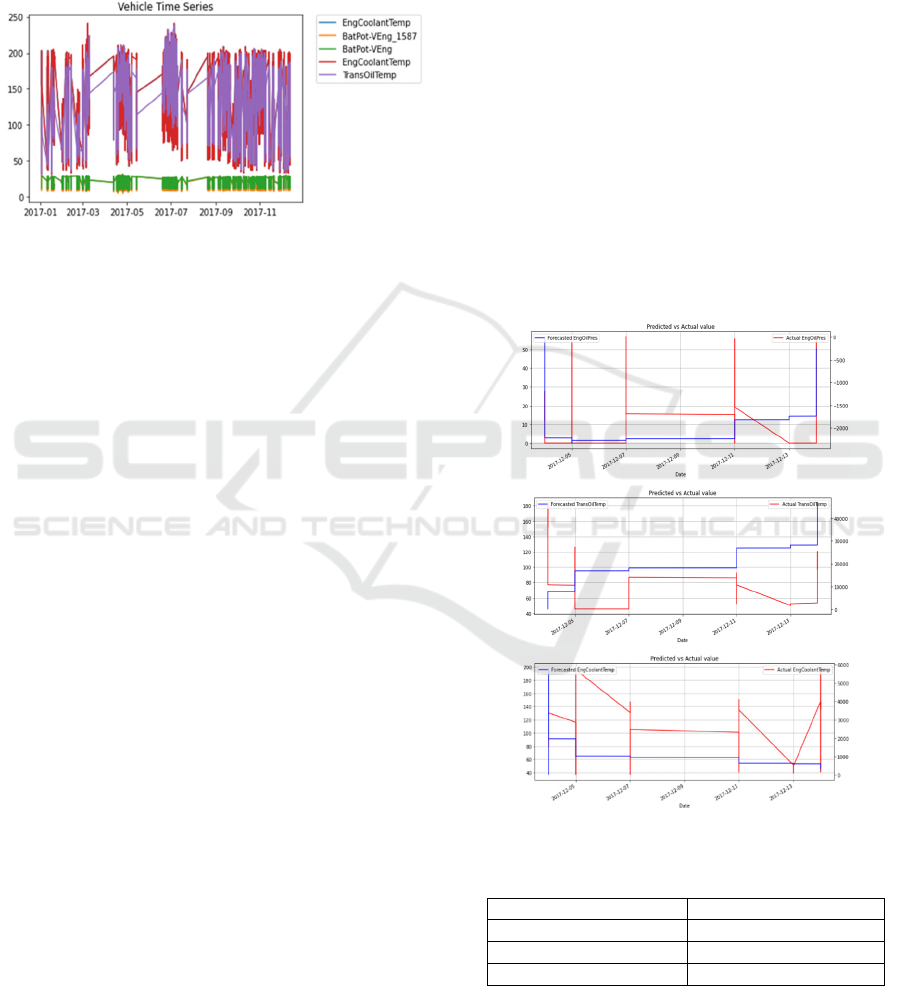
Analyzing the line plot of time series in Figure 5,
we see that all of the time series data follow a
stochastic trend, showing stronger intertemporal
variations with larger drops. All of the series seem to
be related in some way and none look stationary in
their levels. They all appear to have common trends,
an indication that they may be co-integrated.
Figure 5: Time Series line plot.
The series was differenced to make it stationary.
Results from KPSS and ADF tests verified that the
series was difference stationary. The differenced
series was then checked for stationarity. Granger’s
causality test was performed on the first order of the
differenced time series, then tested with 20, 30 and 40
lags applied at 1% and 5% significance levels. P-
values less than the significance levels were found
consistently, confirming the relationships of multiple
variables in the time series and justifying the VAR
modelling approach to forecast the 1Hz operational
dataset.
To determine optimal lag order we have used the
python library model.select_order(maxlags) method
with different values for our max lag. BIC statistics
from running the command suggest the optimal lag
order is 44 and FPE statistics suggest 45. We ran this
command for other VIN numbers and other years, and
the resultant lag order suggestion stayed
approximately the same for all of the data we
considered. Durbin-Watson residual tests indicated
no autocorrelation between the residuals.
We experimented with model VAR model orders
between 42 and 49 for different VIN numbers. In this
paper, we are presenting results from best performing
model. Most models performed best between the lag
length 44-48 and had the lowest number of outliers as
suggested during multivariate outlier analysis. The
worst performing models had RMSE in the range of
40-50% and were discarded.
Before forecasting we de-differenced the
forecasted data once to bring it back to original scale.
Figure 6 shows the plot of forecasted data against
the actual test data for Transmission Oil Temperature,
Engine Coolant Temperature and Engine Oil
Pressure. Forecasting for 8 days was generated using
fitted VAR (44) model in blue. Red represents the
actual value. Forecasted and actual data demonstrate
similar pattern throughout the forecasted days. For
Engine Oil Pressure, forecasted data is close to actual
data but except near transition points. The
Transmission Oil Temperature data pattern is also
very close but predicted values are overestimated.
The Forecast plot for Engine Coolant Temperature
shows a similar pattern, but predicted values were
underestimated for the last two days. In general, we
observed phases of high forecasting accuracy
alternating with phases of low forecasting accuracy.
Identifying structural breaks (Allaro, 2018) in the
data and training the model with segments of time
series is expected to improve forecast accuracy. Table
1 shows the evaluation of VAR model to measure the
average forecast accuracy. RMSE value indicate that
VAR model was not able to successfully forecast
large variation in data therefore it suffered from
accuracy issue.
Figure 6: VAR model forecast data vs. test data.
Table 1: VAR model forecast accuracy.
Variable RMSE
EngCoolantTemp 20.2
EngineOilPressure 17.3
TransOilTem
p
32.3
Data Driven Hybrid Approach for Health Monitoring and Fault Detection in Military Ground Vehicles
305
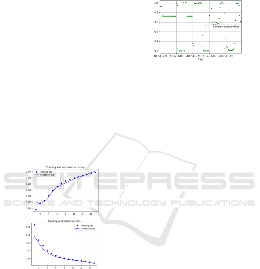
3.2 LSTM Results
Fault detection accuracy varied between the vehicle
models. The entire research effort implemented the
model across several vehicles, but this paper presents
results from building a hybrid VAR-LSTM model for
a single vehicle. The LSTM model that was built
using only historical data provided 65% - 90%
accuracy across multiple vehicles. Once the LSTM
model was built, LSTM model was given the
forecasted VAR data to see if it could detect any fault.
The combined LSTM-VAR model, as a preliminary
finding for a single vehicle, provided at most a 64%
detection accuracy as shown in Figure 7. Therefore,
the LSTM model lost accuracy when detecting faults
as a hybrid model than it did as a stand-alone model.
The loss function in Figure 7 showed a loss of 57%
for this particular vehicle. The LSTM model proved
successful in learning the correlation between normal
operational data and fault data. The LSTM model can
be further expanded to observe data across the entire
vehicle fleet and for an increased period of time. An
increase of time-series data observations and may
contribute to increased model accuracy.
Figure 7: LSTM model training and validation
accuracy/loss.
The hybrid VAR-LSTM model output, produced
scaled fault detection values, labeled as
FailureModeIdentifier, as shown in Figure 8. The
corresponding plot corresponds to the fault values are
indicated as a failure mode value as a function of
time, as shown along the x-axis. These values can be
descaled and traced directly back to the fault code
status log to determine the projected fault status of the
vehicle
.
Figure 8: Hybrid VAR-LSTM model output for fault
detection.
4 CONCLUSIONS AND FUTURE
WORK
The VAR model captured the temporal dynamics of
our time series data but was not able to improve the
accuracy. Experimentation with different VIN
numbers, selection of variable and lag order shows no
signs of improving the VAR model forecast. The
VAR model is a popular tool in time series
forecasting but its parameters are estimated by the
least square technique which is very sensitive to the
presence of outliers. We did not smooth or filter the
outliers from our data because removing the outliers
may disturb the information content hence the series
was only differenced to make it stationary which is a
prerequisite for inferring Granger’s Causality test.
We couldn’t scale the VAR model across the fleet
because this model is computationally expensive to
run and adding more data complicates the learning
ability of the model. We only experimented with a
few variables at a time because adding more variables
to a VAR model creates complications. Predictions
become more unreliable. Another challenge with the
VAR model is that predictions quickly deteriorate.
Very short-term forecasting was found to be slightly
more accurate than long term forecasting, suggesting
some gain is possible by iteratively running the model
over short intervals. In terms of forecast stability, the
model does not constantly yield accurate results
mainly due to structural breaks in the data which can
occur due to periods of inactivity or major
maintenance related change in the vehicle.
Though the LSTM model provided low accuracy
levels using forecasted data, we have succeeded in
building a hybrid workflow for a fault detection
model. However, it can be improved upon with
expanding the model to learn across additional
vehicles and increase the size of the dataset. The
VAR-LSTM hybrid model is very promising for fault
prediction. However, further comparisons of LSTM
DATA 2021 - 10th International Conference on Data Science, Technology and Applications
306

hybrid models should also be evaluated to potentially
increase model accuracy. We will explore other deep
learning models such as CNN-LSTM model (Livieris
et al., 2020), which has been proven successful in
forecasting time series data.
In next phase of the project, in addition to
increasing model sample size, we will be using
corresponding maintenance data for more accurate
forecasting. We will expand our model further using
the fault detection codes to identify data-driven
Remaining Useful Life (RUL) estimation for systems
with abrupt failures. The patterns and trends of
forecasted data our analysis reveals will be used for
condition monitoring and identifying abnormal
operating conditions.
REFERENCES
Allaro HB (2018) A Time Series Analysis of Structural
Break Time in Ethiopian GDP, Export and Import. J
Glob Econ 6: 303. doi: 10.4172/2375-4389.1000303
Akaike, H. (1985), "Prediction and entropy", in Atkinson,
A. C.; Fienberg, S. E. (eds.), A Celebration of Statistics,
Springer, pp. 1–24
Basu, S., Li, X. Q. & Michailidis, G. (2019), ‘Low rank and
structured modeling of high-dimensional vector
autoregressions’, IEEE Transactions on Signal
Processing 67(5), 1207–1222
Dai, X. and Gao, Z. (2013). From Model, Signal to
Knowledge: A Data-Driven Perspective of Fault
Detection and Diagnosis, IEEE Transactions on
Industrial Informatics, vol. 9, (no. 4).
Dickey, D. A.; Fuller, W. A. (1979). "Distribution of the
Estimators for Autoregressive Time Series with a Unit
Root". Journal of the American Statistical Association.
74 (366): 427–431. doi:10.1080/01621459.1979.
10482531
Durbin, J.; Watson, G. S. (1951). "Testing for Serial
Correlation in Least Squares Regression, II".
Biometrika. 38 (1–2): 159–179. doi:10.1093/biomet/
38.1-2.159
Granger, C.W.J. (1980). "Testing for causality: A personal
viewpoint". Journal of Economic Dynamics and
Control. 2: 329–352. doi:10.1016/0165-1889(80)
90069-X
Fu, Y., Huang, D., Qin, N., Liang, K. and Yang, Y. (2018).
High-Speed Railway Bogie Fault Diagnosis Using
LSTM Neural Network, 37th Chinese Control
Conference.
Ha, Y., Chang H. (2018). Forecasting the volatility of stock
price index: A hybrid model integrating LSTM with
multiple GARCH-type models, Expert Systems with
Applications, vol 103.
Hannan, E. J., and B. G. Quinn (1979), "The Determination
of the order of an autoregression", Journal of the Royal
Statistical Society, Series B, 41: 190–195Park, D.C., El-
Sharkawi, M.A., Marks, R.J., Atlas, L.E. and Damborg,
M.J. (1991). Electric load forecasting using an artificial
neural network, IEEE Transactions on Power Systems,
vol. 6, no. 2.
Helbing, G. & Ritter, M. (2018). Deep Learning for fault
detection in wind turbines, Renewable and Sustainable
Energy Reviews, vol 98.
Kwiatkowski, D.; Phillips, P. C. B.; Schmidt, P.; Shin, Y.
(1992). "Testing the null hypothesis of stationarity
against the alternative of a unit root". Journal of
Econometrics. 54 (1–3): 159–178. doi:10.1016/0304-
4076(92)90104-Y
Lee J., Wu F., Zhao W., Ghaffari M., Liao L., Siegel D.
Prognostics and health management design for rotary
machinery systems—Reviews, methodology and
applications Mech Syst Signal Process, 42 (1–2)
(2014), pp. 314-334
Livieris, I.E., Pintelas, E. & Pintelas, P. A CNN–LSTM
model for gold price time-series forecasting. Neural
Comput & Applic. 32, 17351–17360 (2020).
Seabold, S., & Perktold, J. (2010). Statsmodels:
Econometric and Statistical Modeling with Python.
Seth, A. K., Barrett, A. B., & Barnett, L. (2015). Granger
causality analysis in neuroscience and neuroimaging.
The Journal of neuroscience: the official journal of the
Society for Neuroscience, 35(8), 3293–3297.
https://doi.org/10.1523/JNEUROSCI.4399-14.2015
Schwarz, Gideon E. (1978), "Estimating the dimension of a
model", Annals of Statistics, 6 (2): 461–464,
doi:10.1214/aos/1176344136
Zivot, E. and Wang, J. (2006) Vector Autoregressive
Models for Multivariate Time Series. Modeling
Financial Time Series with S-PLUS®. Springer, New
York, NY doi: 10.1007/978-0-387-32348-0_11.
Data Driven Hybrid Approach for Health Monitoring and Fault Detection in Military Ground Vehicles
307
