
Detecting Twitter Fake Accounts using Machine Learning and Data
Reduction Techniques
Ahmad Homsi, Joyce Al Nemri, Nisma Naimat, Hamzeh Abdul Kareem, Mustafa Al-Fayoumi
and Mohammad Abu Snober
Department of Computer Science,
Princess Sumaya University for Technology
, Khalil Al-Saket Street, Amman, Jordan
Keywords: Twitter, ML, Detecting Fake Accounts, Spearman's Correlation, PCA, J48, Random Forest, KNN, Naive
Bayes.
Abstract: Internet Communities are affluent in Fake Accounts. Fake accounts are used to spread spam, give false
reviews for products, publish fake news, and even interfere in political campaigns. In business, fake accounts
could do massive damage like waste money, damage reputation, legal problems, and many other things. The
number of fake accounts is increasing dramatically by the enormous growth of the online social network; thus,
such accounts must be detected. In recent years, researchers have been trying to develop and enhance machine
learning (ML) algorithms to detect fake accounts efficiently and effectively. This paper applies four Machine
Learning algorithms (J48, Random Forest, Naive Bayes, and KNN) and two reduction techniques (PCA, and
Correlation) on a MIB Twitter Dataset. Our results provide a detailed comparison among those algorithms.
We prove that combining Correlation along with the Random Forest algorithm gave better results of about
98.6%.
1 INTRODUCTION
Facebook, LinkedIn, Twitter, Instagram, and other
social media networks, have been growing sharply
over the last century due to technology's growth.
Smartphones, tablets, laptops, and modern devices
helped people in utilizing wireless communication in
in an efficient and easy way. Nowadays, about 4.66
billion people worldwide use the Internet, and 4.14
billion are active users on social media (Johnson,
2021), which represents more than half of the world.
Facebook is considered the biggest online social
network. Facebook has 2.2 billion monthly active
users as of the first month of 2021 (Mohsin, 2021),
whereas Twitter has 330 million monthly active users
and 145 million daily active users (Lin, 2020). Some
of those accounts are fake and lead to misbehaviour,
including political, fake-news-spreading, black-
mailing, misleading ads, terrorist propaganda, spam,
and hate speech. As a result, this will damage the
reputation reliability of the famous Online Social
Networks (OSNs) as fake accounts made it easy to do
such activities.
Online social Networks (OSNs) allow users
having some common ideas to communicate easily.
They are provided the access to many services, such
as: posting comments on their profiles and on the
others’ profiles, messaging and voice/video voice
chatting, buying and selling stuff and services,
sharing news and thoughts and planning/arranging
events.
Moreover, some government entities use OSNs to
provide their driven services, share their official news
and announcements to their citizens, and to share
information about different activities (Awasthi,
Shanmugam, Soumya and Atul, 2020).
A fake profile account is classified into a fake or
duplicated account. We call an account as a
“duplicate” when a user impersonates an account for
another person.
Hiding the real identity for a malicious account for
the reason of malicious activities has grown
dramatically over the last couple of years. The threats
of fake accounts are clustered against one’s reputation
and cause unnecessary confusion by unpredictable
notifications (Awasthi, Shanmugam, Soumya and
Atul, 2020).
Fake profiles, or sometimes called Cyber-Bots,
which are made by cyber-criminals are almost cannot
be distinguished from real accounts, thus makes the
authentication process of user accounts more
complex Some fake accounts are made to
88
Homsi, A., Al Nemri, J., Naimat, N., Abdul Kareem, H., Al-Fayoumi, M. and Abu Snober, M.
Detecting Twitter Fake Accounts using Machine Learning and Data Reduction Techniques.
DOI: 10.5220/0010604300880095
In Proceedings of the 10th International Conference on Data Science, Technology and Applications (DATA 2021), pages 88-95
ISBN: 978-989-758-521-0
Copyright
c
2021 by SCITEPRESS – Science and Technology Publications, Lda. All rights reserved

impersonate a real person’s profile, whereas some
others are made as general accounts to serve as fake
follower (Gurajala, White, Hudson, Voter and
Matthews, 2016).
Machine Learning (ML) algorithms are used to
automate and improve the process of detecting fake
accounts in order to make decisions faster. On the
other hand, bots are also being developed to bypass
those detection algorithms and mechanisms. So, it is
a non-ending battle.
This paper is structured as follows: Section 2
introduces the literature review. Section 3 presents
the methodology used in our work, and Section 4
illustrates the comparison result regarding the
algorithms used. Section 5 shows conclusions and
highlights for future work.
2 LITERATURE REVIEW
Many detection techniques used to classify social
accounts by analysing some existing features. Some
other detection techniques include ML algorithms for
better classifying of accounts.
Authors (Singh, Sharma, Thakral, and
Choudhury, 2018) followed a technique by using
some existing fake accounts to train a machine
learning algorithm. They took a sample size of 20,000
accounts that considered to be fake. In their study,
real accounts had more than 30 followers on average.
So, the first parameter was 30+ followers. The fake
accounts had some prevalent details that certain
individuals adopt to build a fake account, which are:
1. Wrong age for passing eligibility.
2. Incorrect gender definition.
3. Fake image of the profile taken mainly
from the Internet.
4. Image of a gendered character distinct
from the gender set.
5. False Locations for the accounts.
(Khaled, Tazi and Mokhtar, 2018) identified fake
accounts and bots on Twitter by suggesting a new
algorithm. Some machine learning classification
algorithms are used to detect real or fake target
accounts, by using Support Vector Machine (SVM),
Neural Network (NN) algorithms. They combine both
algorithms in a new hybrid one named SVM-NN for a
successful identification of fake accounts. Indeed,
they applied feature selection and dimension reduction
techniques in their work. The accuracy of detecting
fake accounts in their new hybrid algorithm was 98%.
In (Rao, Gutha and Raju, 2020), a cluster
classification approach had been followed which
focused on machine learning. Authors used vector
machines and neural networks to classify fake
accounts. They represent a machine learning pipeline
algorithm to identify fake accounts instead of using
prediction for each account. Their algorithm used to
classify a cluster of Fake accounts if the same person
attempted to generate them. The method started with
selecting profiles to be tested and then extracts the
necessary features and passes them to a trained
classifier along with the feedback. Classifies were
used to classify accounts into fake or real.
In (Isaac, Siodia and Moctezuma, 2016), the
authors suggested a web service that utilized user
accounts and timelines to create an initial feature set
of 71 cheap variables. They separated event-based
highlights into metadata-based and content-based.
Metadata applied to all details on adornment
endorsing or representing the primary substance.
These highlights usually arise from the normal
computation of standard factual. The authors consider
centrality estimators and scattering ratios of less
erratic dispersions in detail. These distributions
include tweet interval rates, tweets spanning over
multiple time ranges, origins of over-posting, and the
sum of intuitive components such as URLs, hashtags,
and tweet mentions. They used feature extraction and
five classification algorithms, which are: random
forest, SVM, Naive bays, Decision tree, and Nnet.
They proved that Random Forest gave the best
accuracy of 94%.
3 RESEARCH METHODOLOGY
This part introduces our proposed model in detail.
Figure 1 shows the model which consists of three
main phases: data preprocessing, data reduction and
data classification. We started our work by processing
the dataset, then we included some reduction
techniques in the second phase. In the reduction
phase, the data was filtered and reduced using some
reduction mechanisms to make it ready for the
classification phase; where the filtered data went
through classification algorithms and the final results
showed up.
Figure 1: Design Approach.
We worked on Weka software, which is a
platform for ML that supports multiple practices of
machine learning in order to implement a proposed
Detecting Twitter Fake Accounts using Machine Learning and Data Reduction Techniques
89

approach or model (Bouckaert, Frank, Hall, Holmes,
Pfahringer, Reutemann, Witten, 2010). Below are the
main features of Weka:
Data Preprocessing: there are a large number of
methods used to filter data, starting from deleting
attributes and ending with more advanced
operations like PCA.
Classification: Weka consists of more than 99
classifiers split into Bayesian, lazy, function-based,
decision tables, tree, misc., and meta, each of which
has a couple of classification algorithms under it.
Clustering: Weka contains many clustering
schemes to support Unsupervised learning, such as
k-means and various hierarchical clustering
algorithms.
Attribute Selection: which consists of a group of
selection criteria and search methods to define the
set of important classes for the classification
performance.
Data Visualization: Data and values resulting from
operations can be represented in understandable
visual graphs.
3.1 Dataset Description
The dataset used in our research is the “MIB” dataset
(Cresci, Pietro, Petrocchi, Spognardi and Tesconi,
2015); which contains 5301 accounts divided as
follows:
3.1.1 Real Accounts
The fake project Dataset contains 469 accounts,
100% human collected in a research project of
researchers at IIT-CNR, in Pisa-Italy.
E13 (elezioni 2013) Dataset contains 1481
accounts all of them are real human accounts, as
they checked by two sociologists from the
University of Perugia, Italy.
3.1.2 Fake Accounts
Fastfollowerz Dataset contains 1337 accounts
Intertwitter Dataset contains 1169 accounts.
Twittertechnology Dataset contains 845
accounts. Those accounts bought by researchers
from the market in 2013.
3.2 Dataset Preprocessing
MIB dataset has two feature of vectors types:
Categorical features: such as name, screenname,
tweets.
Numerical features: such as status-count, friends
count, profile_text_color.
We proceeded by the dataset by considering some
classification algorithms. We also consider the
numerical features types. Moreover, other categorcal
features had been converted into numerical features.
As the dataset contains many attributes, we tried
to test the most significant ones. Attributes that are
not significant were not included in our model. This
is important to apply different ML algorithms on the
dataset (Babatunde, Armstrong, Leng and Diepeveen
2014).
Table 1 lists all the features of the MIB dataset.
Table 1: All Dataset Vectors of the MIB dataset.
1 Profile-lin
k
-colo
r
18 Screen name
2 Profile-background-
colo
r
19 Protected
3 Profile-sidebar-fill-
colo
r
20 Verified
4 Profile-background-
tile
21 Description
5
p
rofile_banner_url 22 Update
d
6 Profile-text-colo
r
23 Dataset
7utc
_
offset 24 created
_
at
8 Default-profile-
image
25 url
9 Default-
p
rofile 26 Lan
g
10 Geo-enable
d
27 time
_
zone
11 Liste
d
-count 28 Location
12 Favourites-count 29
p
rofile_image_url
13 Friends-count 30 Name
14 Followers-count 31 ID
15 Statuses-count 32 profile_image_url
_
https
16 profile_background_
image_url_https
33 profile_backgrou
nd_
image_url
17 Profile-sidebar-
border-color
34 Profile-use-
background-
ima
g
e
After that, we had normalized the data as part of
the data preprocessing phase. The goal here is to
transform the distributed large numerical values to a
common scale of [0,1], without twisting the values
range-differences in order not to lose the information.
In addition, this step is also essential for some
algorithms to model the data appropriately.
When the data distribution is random and
ambiguous or when the distribution is not Gaussian,
then using normalization is a good technique, as
normalization refers to rescaling the selected
attributes from their original values to the scale of 0
DATA 2021 - 10th International Conference on Data Science, Technology and Applications
90

to 1 (Ramos-Pollán, Guevara-López, Suárez-Ortega,
and et al., 2012)
.
3.3 Data Reduction
Principal Component Analysis (PCA) and
Correlation are data reduction methodologies that
used according to their advantages. Some of
advantages of PCA are: removing correlated features,
improving algorithm performance by reducing the
number of features used, reducing overfitting and
improving visualization. While some of the
Correlation advantages are: showing the strength of
the relationship between two variables and gaining
the quantitative data which can be easily analysed.
Here, we describe both techniques in some details.
PCA is a dimensionality reduction method that is
used in the big datasets by converting the large dataset
variables into smaller ones without losing the
information of those values.
The reduction is made by
identifying directions, which is called principal
components, and increase the data variety to the max.
By reducing the number of components, samples
can be shown as small numbers instead of values for
large numbers of variables.
Samples then can be organized in a way which
makes it possible to visually weight differences and
similarities between samples and determine whether
samples can be grouped or not (Ringnér, 2008).
Spearman’s Correlation (aka rho), like all other
Correlation Coefficients, takes two variables (let’s
assume that they are called A and B) and calculates or
measures the strength of connotation between them.
All multi-variable Correlation studies show the
strength of connotation between two variables in a
single value will output a number between -1 and
+1. This output value is called the Correlation
coefficient.
When a positive value of the Correlation
Coefficient shows up, this means that these two
variables have a positive relationship between them
(when the value of variable A increases, the value of
variable B increases). However, when a negative
value of the Correlation Coefficient shows up, this
means that these two variables have a negative
relationship between them (when the value of
variable A increases, the value of variable B
decreases). While, when a value of zero in the
Correlation coefficient shows up, this means that
these two variables have no relationship between
them (Zar, 2014).
The resulted features after processing the dataset
are 15 features. Those features are illustrated in Table
2.
Table 2: Selected Vectors of the Dataset.
1 Profile-lin
k
-colo
r
9 Default-
p
rofile
2 Profile-
b
ackgroun
d
-colo
r
10 Geo-enabled
3 Profile-sidebar-fill-
colo
r
11 Listed-count
4 Profile-
b
ack
g
roun
d
-tile
12 Favourites-count
5 Profile-sidebar-
b
orde
r
-colo
r
13 Friends-count
6 Profile-text-colo
r
14 Followers-count
7 Profile-use-
b
ackgroun
d
-image
15 Statuses-count
8 Default-profile-
ima
g
e
3.4 Data Classification
Classification refers to the process of expecting the
class of provided data points. Sometimes,
targets/labels or categories have the same meaning of
classes. When a mapping function is predicted from
input variables into separate output variables, this
task is called predictive classification modeling.
In learner’s classification, there are two main
types: lazy learners and eager learners.
Lazy Learners. Algorithms work under this
approach are usually save the training data and hold
until the test data show up. After that, we conduct the
classification based on the most of the related data in
the saved training dataset. The time taken by lazy
learners is less, but the predicting time is more than
the eager learner. k-nearest neighbor and Case-based
reasoning are examples of those algorithms.
Eager Learners. In this approach, algorithms usually
build a classification model based on the given
training data to get the classification of the same data.
Eager learners should be able to bind to one
suggestion. This suggestion should cover the whole
instance space. Because of the model construction,
this type takes a long time for training but less time
for prediction. Examples of algorithms use this type
of classification are: Decision Tree, Naive Bayes, and
Artificial Neural Networks.
3.4.1 Classification Algorithms
Nowadays, there are many classification algorithms,
although there is no way to decide which one is better
than the other. It depends on the nature of the dataset
used and the type of the application.
Decision Tree Algorithm is a flowchart
structured-like graph, which considered as a
Detecting Twitter Fake Accounts using Machine Learning and Data Reduction Techniques
91
Supervised learning technique. It can be used for both
classification and regression tasks.
Moreover, it is a statistical-based algorithm where
attributes are selected at the tree-of-nodes beginning
at the root and ending at the leaves. This classification
used to split the data into subsets at each node (leaf)
depending on the attributes’ values (Alsaleh, Alarif,
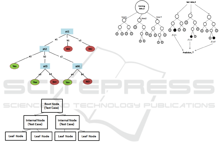
Al-Salman, AlFayez and Almuhaysin, 2014). Figure
2 shows how the Decision Tree works.
J48 was previously named C4.5. It is used to
create a Decision Tree and can be used as a classifier
for the datasets. It is considered also as a statistical
classifier (Xindong, Vipin, Quinlan, Ghosh, Yang,
Motoda , Mclachlan, Ng, Liu, Yu, Zhou, Steinbach,
Hand and Steinberg, 2007). Figure 3 illustrates the
mechanism of J48 classifies.
Figure 2: Decision Tree (Kotsiantis and Sotiris, 2007).
Figure 3: J48 Classifier (Bhargava, Sharma, Bhargava and
Mathuria, 2013).
Random Forest is a machine learning algorithm
that considered as a supervised learning technique. It
creates several Decision Trees on the subset of data.
As well as, it combines each tree prediction to give
the final output prediction for the whole tree based on
all votes technique (Jehad, Rehanullah, Nasir and
Imran, 2012) (Pretorius, Bierman and Steel, 2016).
Moreover, Random Forest is used in Regression and
Classification of ML. It is proved the effectiveness of
this algorithm on large datasets compared to other
classifiers like: Neural Networks, Discriminant
Analysis and Support Vector Machines (SVM)
(Jehad, Rehanullah, Nasir and Imran, 2012).
One of the most important benefits of Random
Forest is that it can work with missing data, which is
the replacement of missing values by the variable that
is common in a particular node. The Random Forest
can also handle big data quickly, provide a higher
accuracy and prevent overfitting problems. One the
other hand, Random Forest requires many computa-
tional resources and large memory for storage, due to
the fact that it creates a lot of trees to save information
piped generated from hundreds of individual trees.
Figure 4 shows how Random Forest works.
Figure 4: Random Forest Classifier (Mennitt, Sherrill and
Fristrup, 2014).
K-Nearest Neighbors (KNN) is one of the
supervised learning techniques. It is used in the
classification and regression tasks, but it is used
especially in the classification. KNN works in two
ways: firstly, the K-Nearest Neighbors pushes a new
data in the training process of the dataset in order to
predict the results. Its classifier is based on just one
point of data that is closest (nearest neighbor)
between all neighboring data points, then the
prediction shows the results as one output. Thus, this
training relies only on one neighbor (Kolahdouzan
and Shahabi, 2004).
In a second way of KNN, all the
closest
neighboring data-points can contribute in assigning a
value called K, which is based on the distance
between test data and a neighbor class such as class A
(Kolahdouzan and Shahabi, 2004). In other words, it
calculates how many neighbors are close and belongs
to class A and how many neighbors are close and
belong to class B, and so on. After selecting the class
with the most belongings, the value of K is computed
and assigned (Mustaqim, Umam and Muslim, 2020).
This method is called “lazy learning” because of its
generalization for the training process of the dataset
after receiving a query on the system. one of the
drawbacks of K-Nearest Neighbors is that it is
sensitive to inconsistent data (noisy) and missing
value data. Figure 5
illustrates how the KNN
classifier works.
DATA 2021 - 10th International Conference on Data Science, Technology and Applications
92
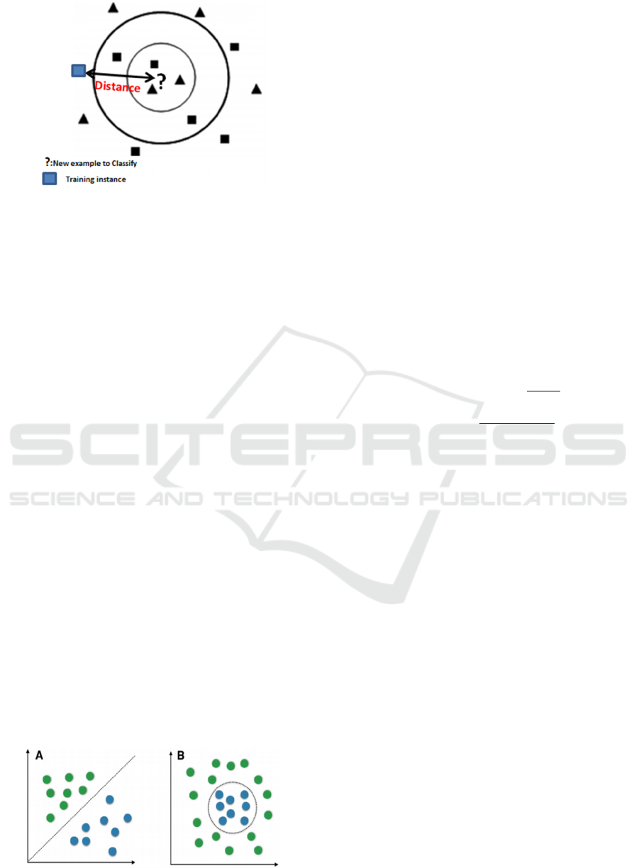
Figure 5: KNN classifier (Moosavian, Ahmadi,
Tabatabaeefar and Khazaee, 2012).
Naive Bayes algorithm is a supervised learning
algorithm which acts as a classifier that can predict
data based on the class observations of the input data.
Also, it gives a probability distribution over many
classes, rather than output the most class that the
observation belongs to (Aridas, Karlos, Kanas,
Fazakis and Kotsiantis, 2019).
In fact, there are some reasons why to choose the
Naive Bayes algorithm:
Fast ML algorithm that does not need much
time in operation, and it is easy to apply to
predict a class from the dataset.
If independent predictors data is correct, the
Naive Bayes performs better than other
algorithms and demand less training dataset.
Naive Bayes is considered as the best
algorithm for categorical variables like text
classification, sentiment analysis (Suppala
and Rao, 2019).
One of the drawbacks for Naive Bayes algorithm
is that it supposes that all features are separated or not
connected. So, we cannot know the relationship
between features. This algorithm faces a challenge
‘zero-frequency trouble’, (i.e. if the categorical
variable has a category in the testing dataset, but not
observed in the training dataset, then the pattern
assigns a 0 probability and will not able to make a
prediction). To overcome this problem, a smoothing
technique shall be used. Figure 6 describes the Naïve
Bayes classifier technique.
Figure 6: Naive Bayes classifier (Raschka, 2014).
4 EXPERIMENTAL RESULTS
AND DISCUSSION
In our experiment, we used the default settings of the
Weka software to determine the training percentage
to be 66% of the whole dataset, and the testing
percentage to be 34%.
The experiment was done by using two reduction
techniques which are: PCA and Correlation, and four
classification algorithms which are: Random Forest,
K-Nearest-Neighbour (KNN), J48, and Naive Bayes.
The data goes into one of the reduction techniques
then all of the four classification algorithms are
applied. For example, the data goes into PCA with
Random Forest algorithm, PCA with KNN algorithm,
and so on.
We have focused in this paper on two
measurements, which are Precision and Accuracy.
Higher Accuracy and precision denotes higher
percentage in detecting fake accounts. These two
measurements can be calculated using the below
equations:
𝑃𝑟𝑒𝑐𝑖𝑠𝑖𝑜𝑛
𝑃𝑅
(1)
𝐴𝑐𝑐𝑢𝑟𝑎𝑐𝑦
𝐴𝐶𝐶
(2)
where, TP: True Positive, FP: False Positive, FN:
False Negative, TN: True Negative.
Our results of combining reduction techniques
along with classification algorithms are shown in
Table 3 and Table 4. In Table 3 where the Correlation
is used with classification algorithms, we observed
that the highest accuracy and precision is achieved
with Random Forest, while we got the lowest
accuracy and precision with Naïve Bayes algorithm
The same observation is deduced from Table 4.
From the same table, we noticed that combining
Correlation with classifier algorithms will give higher
accuracy and precision compared to PCA except the
case Naïve Bayes.
From our results, the highest accuracy was
achieved by using the Correlation reduction
technique along with the Random Forest
classification algorithm with 98.6%. In the second
place, the accuracy of detecting fake accounts was
98% for using Correlation along with J48. Then, the
next higher accuracy is achieved by combining PCA
along with Random Forest with 95.4%. After that, the
PCA along with KNN with 93.56%. Then, the
accuracy of 93.5% goes for using the Correlation
along with KNN. Below that, combining PCA along
with J48 comes with 93.1. Then, the PCA along with
Detecting Twitter Fake Accounts using Machine Learning and Data Reduction Techniques
93
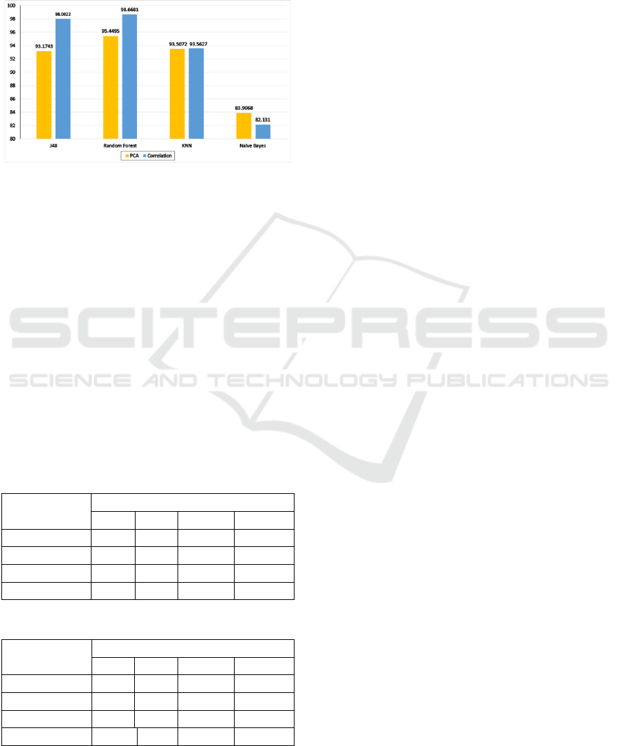
Naive Bayes with an accuracy of 83.9% and lastly
comes the Correlation with Naive Bayes with 82.1%.
Our results are summarized in Figure 7, which
compares the accuracy values of combining both of
the correlation techniques along with all classifier
algorithms used in our study.
Figure 7: Accuracy results for algorithms used.
From the same figure, we conclude that in order
to get the most accurate and precise result we have to
combine Correlation technique with Random Forest
algorithm. However, using the Correlation technique
along with Naive Bayes algorithm leads to the lowest
accuracy and precision. In addition, our results show
that the use of any of the correlation techniques along
with KNN algorithm has almost no effect regarding
the accuracy and precision.
Moreover, the Naive Bayes algorithm is the only
classifier that gives a lower accuracy when combined
with the any of the Correlation technique compared
with all other algorithms. The reason goes back where
the Naïve Bayes algorithm performance is decreased
when data features are highly correlated.
Table 3: Overall Results of our experiment using
Correlation.
Correlation
TP FP Precision Accuracy
J48 0.980 0.029 0.980 98.0022
Random Forest 0.987 0.014 0.987 98.6681
KNN 0.936 0.083 0.935 93.5627
Naive Bayes 0.821 0.262 0.827 82.131
Table 4: Overall Results of our experiment using PCA.
PCA
TP FP Precision Accuracy
J48 0.932 0.080 0.932 93.1743
Random Forest 0.954 0.047 0.955 95.4495
KNN 0.935 0.081 0.935 93.5072
Naive Bayes 0.839 0.215 0.838 83.9068
5 CONCLUSIONS AND FUTURE
WORK
In this study, we aimed at studying the effect of two
correlation techniques along with some ML
algorithms. Our main goal is to get a better
understanding of the effects of the correlation with
the classifier algorithms in detecting fake accounts on
social media. Our work is based on MIB dataset and
done using Weka software. The data preprocesing
and reduction phases of our model were designed to
make the dataset applicable for the classification
process. After that, the data went through the
classification phase to determine the best accuracy
along with different machine learning algorithms.
For the data reduction phase, the Principal
Component Analysis (PCA) and Correlation were
used with four classifier algorithms, which are: J48,
Random Forest, KNN, and Naive Bayes. Results
show that Random Forest algorithm along with
Correlation data reduction gives the best accuracy of
98.6%. While Naive Bayes algorithm along with
Correlation data reduction achieve the lowest
accuracy of 82.1%.
There are still many different experiments and
methodologies and algorithms need to be tested and
are left for the future. We plan to use different
reduction techniques and to test different
classification algorithms by doing deeper
investigation and analysis.
REFERENCES
Johnson, J., 2021 Jan 27, Global digital population,
https://www.statista.com/statistics/617136/digitalpopu
lation-worldwide/
Mohsin, M., 2020 May 10, 10 Facebook Statistics Every
Marketer Should Know In 2021[INFOGRAPHIC],
https://www.oberlo.com/blog/facebook-statistics
Lin, Y., 2020 May 30, 10 Twitter Statistics Every Marketer
Should Know In 2021 [INFOGRAPHIC], https://www.
oberlo.com/blog/twitter-statistics
Awasthi, S., Shanmugam, R., Soumya, J., Atul, S. (2020).
Review of Techniques to Prevent Fake Accounts on
Social Media. International Journal of Advanced
Science and Technology. 29. 8350-8365
Gurajala, S., White J., Hudson, B., Voter, B., Matthews J.
(2016). Big Data & Society DOI: 10.1177/205
3951716674236
Singh, N., Sharma, T., Thakral, A., Choudhury, T. (2018).
Detection of Fake Profile in Online Social Networks
Using Machine Learning. 231-234. 10.1109/ICACCE.
2018.8441713.
DATA 2021 - 10th International Conference on Data Science, Technology and Applications
94

Khaled, S., El-Tazi, N., Mokhtar, H. (2018). Detecting Fake
Accounts on Social Media. 2018 IEEE International
Conference on Big Data (Big Data).
doi:10.1109/bigdata.2018.862191
Rao, K., Gutha, S., Raju, B. (2020). Detecting Fake
Account On Social Media Using Machine Learning
Algorithms. International Journal of Control and
Automation. 13. 95-100
Isaac, D., Siordia, O., Moctezuma, D., (2016). Features
combination for the detection of malicious Twitter
accounts. 1-6. 10.1109/ROPEC.2016.7830626
Bouckaert, R., Eibe, F., Hall, M., & Holmes, G.,
Pfahringer, B., Reutemann, P., Witten, I. (2010).
WEKA—experiences with a Java Open-Source Project.
Journal of Machine Learning Research.
Cresci, S., Pietro, R., Petrocchi, M., Spognardi, A., Tesconi,
M. (2015). Fame for sale: efficient detection of fake
Twitter followers. arXiv:1509.04098 09/2015. Elsevier
Decision Support Systems, Volume 80, Pages 56–71.
Babatunde, O., Armstrong, L., Leng, J., Diepeveen, D.
(2014). A Genetic Algorithm-Based Feature Selection.
International Journal of Electronics Communication
and Computer Engineering, 5(4), 899-905
Ramos-Pollán, R., Guevara-López, M.A., Suárez-Ortega,
C. et al. (2012) Discovering Mammography-based
Machine Learning Classifiers for Breast Cancer
Diagnosis. J Med Syst 36, 2259–2269 (2012).
DOI:10.1007/s10916-011-9693-2
Ringnér M. (2008) What is principal component analysis?
Nat Biotechnol. Mar;26(3):303-4. doi: 10.1038/nbt030
8-303. PMID: 18327243.
Zar, J. (2014). Spearman Rank Correlation: Overview.
Wiley StatsRef: Statistics Reference Online
Alsaleh, M., Alarif, A., Al-Salman, A., AlFayez, M.,
& Almuhaysin, A. (2014). TSD: Detecting Sybil
Accounts in Twitter. 2014 13th International
Conference on Machine Learning and Applications,
462-469. doi:10.1109/ICMLA.2014.8
Kotsiantis, S. (2007). Supervised Machine Learning: A
Review of Classification Techniques. Informatica
(Ljubljana). 31.
Xindong, W., Vipin, K., Quinlan, R., Ghosh, J., Yang, Q.,
Motoda, H., Mclachlan, G., Liu, B., Yu, P., Zhou, Z.,
Steinbach, M., Hand, D., Steinberg, D., (2007). Top 10
algorithms in data mining. Knowledge and Information
Systems. 14. 10.1007/s10115-007-0114-2.
Bhargava, N., Sharma, G., Bhargava, R., Mathuria, M.
(2013). Decision Tree Analysis on J48 Algorithm for
Data Mining. International Journal of Advanced
Research in Computer Science and Software
Engineering Volume 3, Issue 6, (2013 June). ISSN:
2277 128X
Jehad, A., Rehanullah, K., Nasir, A., Imran, M. (2012 SEP).
Random Forests and Decision Trees. International
Journal of Computer Science Issues (IJCSI). vol 9,
Issue 5, No. 3. 1694-0814
Pretorius, A., Bierman, S., Steel, S. (2016). A meta-analysis
of research in random forests for classification. IEEE
Conference 2016. 1-610.1109/RoboMech.2016.78131
71
Mennitt, D., Sherrill, K., Fristrup, K. (2014). A geospatial
model of ambient sound pressure levels in the
contiguous United States. The Journal of the Acoustical
Society of America (2014 MAY). DOI:
10.1121/1.4870481
Kolahdouzan, M., Shahabi, C. (2004). Voronoi- Based K
Nearest Neighbor Search for Spatial Network
Databases. Proceeding of the 30th VLDB Conference.
30. 840-851. 10.1016/B978-012088469-8.50074-7.
Mustaqim, T., Umam, K., Muslim, M. (2020). Twitter text
mining for sentiment analysis on government’s
response to forest fires with vader lexicon polarity
detection and k-nearest neighbor algorithm. Journal of
Physics: Conference Series 1567. 032024. DOI:
10.1088/1742-6596/1567/3/03202
Moosavian, A., Ahmadi, H., Tabatabaeefar, A., Khazaee,
M. (2012). Shock and Vibration 20 (2013) 263–272
263. DOI 10.3233/SAV-2012-00742blog/2016/6/4/
time-series-analysis-fitbit-using-dtw-and-knn
Aridas, C., Karlos, S. Kanas, V. Fazakis, N. Kotsiantis, S.
(2019). Uncertainty Based Under-Sampling for
Learning Naive Bayes Classifiers Under Imbalanced
Data Sets. IEEE Access. PP(99). 1-1. DOI:10.1109/
ACCESS.2019.2961784
Suppala, K., Rao, N. (2019). Sentiment Analysis Using
Naive Bayes Classifier. International Journal of
Innovative Technology and Exploring Engineering
(IJITEE) ISSN: 2278-3075, Volume-8 Issue-8 June,
2019.
Raschka, S. (2014). Naive Bayes and Text Classification.
arXiv:1410.5329v4 (Feb 2017).
Detecting Twitter Fake Accounts using Machine Learning and Data Reduction Techniques
95
