
Synthesizing Fundus Photographies for Training Segmentation Networks
Jannes S. Magnusson
1,∗ a
, Ahmed J. Afifi
2 b
, Shengjia Zhang
3 c
, Andreas Ley
2
and Olaf Hellwich
2
1
Institute of Computer-assisted Cardiovascular Medicine, Charit
´
e–Universit
¨
atsmedizin Berlin,
Augustenburger Platz 1, 13353 Berlin, Germany
2
Computer Vision and Remote Sensing, Technische Universit
¨
at Berlin, Marchstr. 23, 10587 Berlin, Germany
3
Shanghai Key Laboratory of Digital Media Processing and Transmission, Shanghai Jiao Tong University,
800 Dongchuan Rd., Minhang District, Shanghai, China
Keywords:
Fundus Image Synthezis, Retina Vessel Segmentation, Convolutional Neural Networks, ResNet, U-Net.
Abstract:
Automated semantic segmentation of medical imagery is a vital application using modern Deep Learning
methods as they can support clinicians in their decision-making processes. However, training these models
requires a large amount of training data which can be especially hard to obtain in the medical field due to
ethical and data protection regulations. In this paper, we present a novel method to synthesize realistic retinal
fundus images. The process mainly includes the vessel tree generation and synthesis of non-vascular regions
(retinal background, fovea, and optic disc). We show that combining the (virtually) unlimited synthetic data
with the limited real data during training boosts segmentation performance beyond what can be achieved
with real data alone. We test the performance of the proposed method on the DRIVE and STARE databases.
The results highlight that the proposed data augmentation technique achieves state-of-the-art performance and
accuracy.
1 INTRODUCTION
Fundus photography is used for important medical
examinations of the retina to notice different dis-
eases early, such as age-related macular degenera-
tion, diabetic retinopathy, glaucoma, and many oth-
ers (Abr
`
amoff et al., 2010). A large number of algo-
rithms for optic disc (OD) detection, vessel segmenta-
tion, and width measurements were developed in or-
der to help clinicians with the diagnosis of diseases
(Patton et al., 2006). Among those methods, vessel
segmentation is a tough task due to varying vessel
sizes, low contrast images, and differences in the ap-
pearance of diseases like microaneurysms and hemor-
rhages (Liskowski and Krawiec, 2016a). Overcoming
these challenges may improve the diagnosis process
of different diseases.
To solve the retinal vessel segmentation (RVS)
task, deep learning plays a significant role in recent
approaches. Different neural network architectures
were proposed to solve this problem (see Section 2.2).
a
https://orcid.org/0000-0002-3913-735X
b
https://orcid.org/0000-0001-6782-6753
c
https://orcid.org/0000-0001-7664-6500
∗
Corresponding author
Figure 1: The pipeline of the proposed method. In three
almost independent tasks, the image is generated piece by
piece, merged, and applied to general adjustments of illu-
mination, intensity, etc.
The main issue that was tackled is the issue of seg-
menting tiny vessels correctly ((Soomro et al., 2017),
(Feng et al., 2020)). Many methods introduced a large
and complex preprocessing pipeline to improve the
input image characteristics like contrast and illumina-
tion combined with data augmentation. This under-
Magnusson, J., Afifi, A., Zhang, S., Ley, A. and Hellwich, O.
Synthesizing Fundus Photographies for Training Segmentation Networks.
DOI: 10.5220/0010618100670078
In Proceedings of the 2nd International Conference on Deep Learning Theory and Applications (DeLTA 2021), pages 67-78
ISBN: 978-989-758-526-5
Copyright
c
2021 by SCITEPRESS – Science and Technology Publications, Lda. All rights reserved
67

lines the actual problem. There are databases avail-
able to use for training. They are mostly limited to
very few images (20 for STARE (Hoover et al., 2000),
40 for DRIVE (Staal et al., 2004)). Each image had
to be labeled by hand. Labeling one image needs
to be done by an expert for several hours (Hoover
et al., 2000) which makes gathering data very expen-
sive. Additionally, medical data is always linked to
patient privacy (Guibas et al., 2017). This limited
amount of images cannot fulfill the requirement of
sufficient training data of an accurate segmentation
network based on deep learning. Synthesizing fun-
dus images can overcome this problem and provide a
flexible environment to generate more data for train-
ing and validation.
In the past, some approaches were developed to
generate synthetic data. (Fiorini et al., 2014) and
(Zhao et al., 2018) only focus on generating synthetic
backgrounds by using real vessel trees. (Costa et al.,
2017b) provides a generation method for vessel trees
which produces unrealistic vessel trees with recoiling
branches and a little number of tiny vessels. Tiny ves-
sels are the main challenge in retinal vessel segmen-
tation. Synthetic data must therefore provide a de-
cent amount of tiny vessels to be sufficient for well-
performing segmentation approaches.
The main contribution of the presented work is a
complete pipeline to synthesize realistic retinal fun-
dus images based on observations to the DRIVE
database. Figure 1 shows the pipeline of the proposed
synthesizing method. It mainly includes three parts:
• the generation of the vessel tree by a novel ap-
proach which overcomes the limitation of statisti-
cal models based on limited available data
• synthesizing non-vascular regions (optic disc,
background, and fovea)
• merging all components and adding final tone
mapping
The advantage of this method is the focus on tiny
vessels to improve their segmentation. Lastly, it is
shown that data augmentation based on the synthetic
images achieves state-of-the-art performance in RVS
for DRIVE and STARE databases. The algorithm
and final trained networks are publically available on
github
1
.
2 STATE-OF-THE-ART
Starting with state-of-the-art methods on retinal im-
age synthesis gives an overview of problems that are
1
https://github.com/jannessm/RetinaSynthesis
tackled by the presented method. To evaluate our
method, the impact in retinal image segmentation
must be discussed. Therefore, current progress in reti-
nal vessel segmentation is stated in the following.
2.1 Retinal Image Synthesis
The conventional approach of image synthesis tries
to find mathematical models to describe image for-
mation and its characteristics. These can either be
based on anatomical knowledge or on statistical dis-
tributions and deviations.
The retinal image consists of three main elements:
the optic disc, the fovea, and the vascular network. A
complete process must synthesize all of them plus the
orange-red retinal tissue in the background. For the
generation of the background and the fovea, Fiorini
et al. (Fiorini et al., 2014) proposed a patch-based
approach, in which a color intensity distribution map
and its corresponding clustering map are constructed
from real images to build a dictionary of tiles for syn-
thesizing images. Additionally, Fiorini et al. (Fiorini
et al., 2014) developed a parametric intensity model
for the optic disc generation. The parameters were
estimated over 30 images from the High-Resolution
Fundus (HRF) Image Database (Budai et al., 2013).
Bonaldi et al. (Bonaldi et al., 2016) used an Ac-
tive Shape Model to extract the skeleton. A statistical
representation of landmarks on the image was devel-
oped. A spatial density distribution map of these land-
marks was used to generate bifurcation points. Mur-
ray’s Law is used to determine the angle and diameter
of branches.
Zhao et al. developed another GAN approach to
generate synthetic images according to a given ves-
sel tree (Zhao et al., 2018) similarly as (Costa et al.,
2017a).
A purely data-driven method has been proposed to
generate synthetic retinal images by deep learning ap-
proach (Costa et al., 2017b). An adversarial autoen-
coder is implemented to generate vessel networks fol-
lowed by a generative adversarial network (GAN) to
generate background, fovea, and optical disc accord-
ing to the vessel tree.
This brief overview stresses the lack of complete
pipelines of generating synthetic images including
synthetic vessel trees. The main issue of the usage of
deep learning-based approaches for vessel tree gener-
ation is that the density of vessels sometimes is too
high, some branches recoil, and the amount of tiny
vessels is less than for real images. Therefore, a
model is presented in the following to generate im-
ages with tiny vessels and an accurate representation
of these in the ground truth.
DeLTA 2021 - 2nd International Conference on Deep Learning Theory and Applications
68

2.2 Segmentation
Medical image analysis aims to develop auxiliary
tools e.g. algorithm-based computer software to help
clinicians to make better diagnoses and therapy plans.
Many approaches have been proposed to solve the
problem of retinal vessel segmentation (RVS). The
first publication in 1989 uses Gaussian-shaped distri-
butions to approximate the gray-level profile and by
filter matching, vessel segments are detected (Chaud-
huri et al., 1989). By then many publications ad-
dressed RVS in different ways. Some approaches
used hand-crafted features like pixels’ maximal gra-
dient and curvature in scale-space (Mart
´
ınez-P
´
erez
et al., 1999), or an active contour model which was
grown along vessels for detection (Al-Diri et al.,
2009).
With the growth of successes in deep learning, the
segmentation problem was addressed by neural net-
works (Soomro et al., 2019b). In 2015, Zhang et al.
(Zhang et al., 2015) trained a two-layer competitive
neural network (Kohonen’s self-organizing map) but
still, the average accuracy was only almost as good
as the human observer (see Table 2). In the same
year, another approach used a simple convolutional
network with 5 convolutional layers. It outperforms
the previous method but still performs worse than the
human observer used as the gold standard (Melin
ˇ
s
ˇ
cak
et al., 2015). In 2016, a very similar architecture was
used (4 convolutional layers with less max-pooling
than the previous work) and introduced a large pre-
processing pipeline including contrast normalization
and whitening. For data augmentation, not only sub-
sampling was used but also different transformations
like rotation and scaling (Liskowski and Krawiec,
2016b). These steps improved specificity and accu-
racy beyond the human observer. Far less successful
was the attempt to use a two-stage binarization by Yao
et al. (Yao et al., 2016). The enhanced green channel
of the input sample and a prediction of a CNN with 3
convolutions were combined into a final segmentation
result.
Ngo and Han presented a multi-level CNN archi-
tecture in 2017 that used two scales of the image as
an input (Ngo and Han, 2017). Therefore, the high
detail in the large input could be combined with the
overall context from the large image. Soomro et al.
(Soomro et al., 2017) focused on both, using more ad-
vanced CNN architectures and improving the prepro-
cessing pipeline to enhance the feature quality that is
passed to the CNN. They used an encoder-decoder ar-
chitecture inspired by the success of the SegNet. For
preprocessing the image, morphological methods and
color-to-grey conversions based on PCA were used.
Later on, they showed that a modified version of the
U-Net in combination with the dice-loss further im-
proved the results (Soomro et al., 2019a). The ad-
vantage of the dice-loss is the consideration of unbal-
anced classes, like in this case. Vessels only appear
in 10% of all pixels (Soomro et al., 2017). (Hu et al.,
2018), (Wang et al., 2019), (Feng et al., 2020), and
(Zou et al., 2020) followed the approach of using pre-
vious features and combining these with deeper ones
in the neural network architecture. These achieved
state-of-the-art results. Since this paper focuses on
the generation of synthetic images, the success of U-
Net like architectures is used to prove the applicability
of the presented method.
However, the most prominent issue is missing out
on tiny vessels in the retinal images, which are hard
to detect. Often humans do not agree on the presence
of the tiniest vessels in the image. This and the limit
of available data is crucial for segmenting tiny vessels
based on deep learning. To improve the training pro-
cedure in segmentation, image synthesis is a good and
practical way to augment databases.
3 SYNTHESIS
The process of image synthesis involves two parts.
Firstly, the background with the fovea, optic disc,
and vessel trees are generated separately. Afterward,
those are combined into one image and a mask from
the DRIVE database is used to create the circular
crop. The combination is done by the Porter Duff
Composition (Porter, 1984). Examples of the final
images can be seen in Figure 2. It is obvious to the hu-
man eye that these images are artificial but the results
show that the most important aspects to improve seg-
mentation are included. In contrast to the deep learn-
ing methods of (Zhao et al., 2018) and (Costa et al.,
2017b) additional variance of vessel trees and back-
grounds are added that are not included in the limited
amount of real data.
3.1 Background and Fovea
To generate realistic backgrounds for retinal images,
Perlin noise is used with five different octaves for pro-
ducing a non-uniform texture of the background. For
the fovea part, a simple circle will be colored by a
dark gradient. This results in smooth transitions be-
tween the fovea and the texture produced by the Perlin
noise. The color ranges are chosen on the basis of the
DRIVE database.
Synthesizing Fundus Photographies for Training Segmentation Networks
69

Figure 2: Examples of the generated synthetic images
created by the proposed method with their corresponding
ground-truths. In this overview, the different random pa-
rameters like mirroring or color ranges of the image are
clearly visible.
3.1.1 Texture
Perlin noise (Perlin, 2002) is used to generate the
background texture. It is a powerful method that is
often used in procedural content generation. Here, the
two-dimensional Perlin noise is implemented follow-
ing (Perlin, 2002). A pseudo-random gradient vector
is generated and interpolated by the quintic function
6t
5
− 15t
4
+ 10t
3
. This is proposed to overcome arti-
facts. Furthermore, a mixture of five octaves P( f req)
with different amplitudes are used depending on the
size of s of the image which improves the result:
Texture = 0.1P(
s
8
) + 0.1P(
s
16
) + 0.1P(
s
32
)
+ 0.2P(
s
64
) + 0.3P(
s
128
)
(1)
3.1.2 Fovea
It can be seen in Figure 1 that the fovea appears as
a darker spot in the center of the image. Hence, it
is sufficient to use a gradient in that area that alters
the intensity of the texture generated before. This is
achieved by the following formulas.
dist(x,y,x
0
,y
0
,r) =
min
(x − x
0
)
2
+ (y − y
0
)
2
r
2
,1
(2)
f (x,y,x
0
,y
0
,r) = 0.5 +
3dist − 2dist
3
2
2
(3)
Figure 3: The RGB value distributions of the optic disc of
a sample from the DRIVE database (from top to bottom:
R, G, B; from left to right: original image, mathematical
model). The discontinuity in the left images is the result of
removing vessels in the optic disc area as shown in Figure
4.
Equation 2 calculates the distance to the center of
the fovea (x
0
,y
0
) which is chosen randomly. r denotes
the radius of the fovea which is picked according to
the anatomical characteristics. Equation 3 uses this
distance to create an intensity factor in the range of
[0.58,1]. This factor is applied to each color channel.
3.2 Optic Disc
The optic disc has a yellow circular shape. More pre-
cisely, it is made up of an inner circle and an outer
circle. Both of them are brighter than other structures
in the image and the inner circle is brighter than the
outer circle.
To analyze the most significant aspects of the op-
tic disc, the color distribution of the retinal image in
three color channels is plotted in Figure 3. It stresses
that red values form a mountain with a flat hilltop.
The surface of green values and blue values have a
cone-shaped structure on the top of a shape that is
similar to the previous red value surface. To synthe-
size the optic disc, the method from (Fiorini et al.,
2014) is adopted to calculate color values (Equation
4 and Equation 7). Because the distribution of green
values and blue values are almost the same, they share
the same mathematical model.
R(x,y, p
r
) = z
0
+
1
a
0
+ exp[l − m]
(4)
where l and m are defined as
DeLTA 2021 - 2nd International Conference on Deep Learning Theory and Applications
70
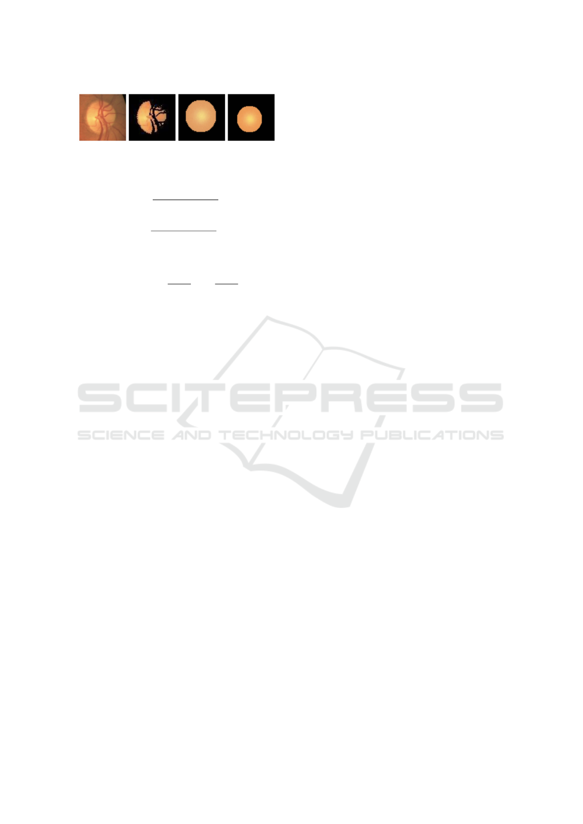
Figure 4: From left to right: real retinal image, segmented
optic disc (after removing vessels), randomly synthesized
optic disc 1, and the randomly synthesized optic disc 2.
l = −(
x − x
0
+ cos(wφ)
σ
x
)
2
(5)
m = (
y − y
0
+ cos(wφ)
σ
y
)
2
(6)
GB(x,y,p
gb
,q
gb
) = R(x,y, p
gb
)
− kexp
−(
x − x
1
σ
x
1
)
2
− (
y − y
1
σ
y
1
)
2
(7)
In these equations, p
r
= [z
0
,a
0
,x
0
,y
0
,σ
0
], p
gb
=
[z
1
,a
1
,x
1
,y
1
,σ
1
], and q
gb
= [k,x
2
,y
2
,σ
2
] are the cor-
responding parameter sets. z denotes the base color
value. a denotes how large the plain area on the hill-
top is. (x
0
,y
0
) describes the center of the inner circle
and the outer circle of the optic disc. σ denotes the
degree of spread or scatter. k denotes the height of the
cone-shaped structure and φ = arctan(y − y
0
,x − x
0
).
They are all estimated by fitting the model to real im-
ages using a non-linear least squares regression. To
eliminate the influence of the vessels over the optic
disc whose colors are darker, the optic disc is ex-
tracted. Then the model is fitted to this extracted
area as shown in Figure 4. The position of the op-
tic disc is determined by the fovea’s position and the
distance between them according to medical knowl-
edge (Patzelt, 2009). By adding small and reasonable
random offsets to each parameter, many different op-
tic disc images can be generated.
3.3 Vessels
The vessel tree is generated in three steps. Firstly,
a starting and target point for each vessel has to be
determined. Then the path between those points has
to be generated to display each pixel. Finally, the path
is drawn on an image. In the following, the horizontal
image size is denoted as h. In contrast to the method
of Castro et al. (Castro et al., 2020), various levels of
vessels are distinguished to enhance the control over
each level.
3.3.1 Select Target Points
For selecting a target point, three levels of branches
are differentiated. Each level follows a different
heuristic. The first level vessels are the main branches
starting from the center of the optic disc. There are
four vessels for arteries and four for veins. Each ves-
sel leads to one edge of the image. To randomize
the resulting branches, for each vessel a random point
from a specific area in each corner of the image is se-
lected. These regions are either left to the fovea or
right to the optic disc, assuming that the optic disc
is always right to the fovea. The regions left to the
fovea are therefore determined by the location of the
fovea. The regions right to the optic disc are selected
according to the position of the optic disc and the im-
age dimensions. All values are selected empirically
with the assumption that the main vessels have to go
beyond the boundaries of the image.
For the second level (the subbranches of the main
vessels), the position on the starting point on the main
vessel is analyzed and a new target point is selected.
The calculation of this new target point differs be-
tween points on the left of the optic disc and on the
right of the optic disc.
If the starting point is left to the optic disc, either
the new vessel grows to the fovea or away from it.
But for both opportunities, the new x coordinate is
to the left of the starting point. Therefore, the main
direction of the new vessel differs less than 90
◦
to the
main direction from the parent. This is important to
ensure realistic blood flow. The y direction is either
almost at the fovea (with a probability of 0.5) or the
y position of the starting point added with a random
number j ∈ [40,0.3h]. As a reminder, h denotes the
image width.
For the second case for the second level of
branches (the starting point lies right to the optic
disc), the direction vector from the starting point to
the target point of the parent vessel is normalized
to a length of 1, then rotated by α ∈ [30
◦
,70
◦
], and
stretched to the length l ∈ [40,0.3h].
The last heuristic covers all levels higher than
level 2. In this method, a window w with a size s
of the binary image of the tree is analyzed around the
starting point p
s
. All regions between vessels in w
are segmented and labeled uniquely. If a region con-
tains more than 1% of the image size and is directly
located next to the parent vessel of p
s
, the center c
of this region is considered as a candidate for a new
target point. Additionally, only candidates are consid-
ered, where the path from p
s
to c does not cross any
other vessel. If candidates were found, the center of
the largest region is selected as a final candidate. To
prevent parallel vessels, the angle between p
s
to the
parent’s target point, and from p
s
to the final candi-
date needs to be higher than 20
◦
.
To get a center of a large area, the size of the
Synthesizing Fundus Photographies for Training Segmentation Networks
71

Figure 5: In the left setup, the vessel needs to move around the fovea. Starting at the current point x. ~r is rotated by θ to x
0
.
With respect to the baseline from x to x
0
, x
0
is again rotated by a random angle ∈ [−30
◦
,30
◦
]. This results in a next point i
which is added to the current vessel. In the right setup, the baseline can be set straightforward to the target point. Resulting in
point i after the same rotations θ and by an random angle as in the left setup.
window s is increased until the maximum of 2h/3 is
reached or a candidate moved more than 3 px in an
increasing step. The movement indicates that two re-
gions have merged because of the increased width of
the window.
3.3.2 Determine the Vessel Path
To imitate realistic retinal vessels, a curly vessel path
is required. Additionally, the vessels need to curve
around the fovea at first and then head to the target
point.
The positions of the fovea, the target point y, and
the current point x are used to determine a new and
next point i which is at a random distance of l. The
vector from the fovea to x is called~r, the vector from
the fovea to y is called ~r
g
and ~r
i
is the vector from the
fovea to i. Two situations are discriminated, either the
angle between ~r and ~r
g
is larger than 90
◦
or smaller
than 90
◦
. Both situations are visualized in Figure 5.
In the first situation, x is near the starting point.
An angle θ is calculated based on l and |~r| in Equa-
tion 8. Parameter ε is introduced to add randomness.
Then~r is rotated by θ towards y. The endpoint is de-
noted as x
0
so that the vector from x to x
0
is denoted as
~
x
0
. Afterwards,
~
x
0
is rotated in a range of [−30
◦
,30
◦
]
to get the final direction to i so that the vessel path
appears curly. At last, i is determined with a distance
l from x (see left sketch of Figure 5).
θ =
l
|~r| + ε
,ε ∈ [−20,10] (8)
In the second situation as shown on the right in
Figure 5, the baseline is directly set from x to y and
the location of i is determined within an angle range
of [−30
◦
,30
◦
] and distance of l from x.
The method is repeated until the distance between
x and y is smaller than a threshold of 0.03h or x is out
of the image.
3.3.3 Drawing Vessels
To create colored images from the points generated
along a vessel, all points are interpolated by a cubic
spline. Next, colors are selected and widths are de-
termined along the path. From the target point to the
starting point the width is increased by Equation 9.
This function increases the width for every i-th point
on the path by α, starting from a diameter of d pt.
Each level of vessels has its own α and d which en-
sures realistic diameters.
f (x) =
α · i
h
+ d
h
565
(9)
For the colors, different values for arteries and
veins are chosen empirically by comparing the result
with real images. Arteries are colored with a RBGA
value of (150, 30, 10, t) and veins have a color of (110,
10, 5, t). t determines the transparency of the vessel
so that the ends of vessels will disappear slowly as can
be noticed in real fundus photographies.
3.4 CNN Architecture and Training
Details
The underlying architecture is based on a modified
encoder-decoder architecture called Res-U-Nets. A
similar architecture was used by (Ibtehaz and Rah-
man, 2020) which has shown great performance on
medical segmentation tasks. One difference to our
network is that residual blocks are used within the en-
coder and decoder (Figure 6) instead of normal con-
volutions. Furthermore, (Ibtehaz and Rahman, 2020)
adds other residual convolutions in the connection
from the encoder to the decoder where the used net-
work does not further process the data on these con-
nections. The last difference is the inclusion of two
downsampling and upsampling blocks in the encoder
DeLTA 2021 - 2nd International Conference on Deep Learning Theory and Applications
72

Figure 6: The architecture used to evaluate the generated synthetic images on the left. The purple and blue blocks represent
residual blocks for encoder and decoder respectively from the right of this figure. At the top, one can see the encoder, whereas
the bottom describes a decoder block.
and decoder. The whole network can be seen in Fig-
ure 6 which outlines the U-Net shape and refers to the
special residual network blocks in different colors.
The resulting network is trained on patches of size
128 × 128 pixels with basic data augmentation pre-
processing including random brightness, contrast, and
noise to gain robustness in the predictions. Through
the limitation of real images, the main goal of the
training process is to retrieve all important statistics
from these images which are learned by the first lay-
ers. For all deeper layers, it is important to learn the
overall structure of retinal images. This is covered
well by the generated, synthetic images. Therefore,
the proposed training process uses mini-batches of 32
items including 16 synthetic and 16 realistic patches
of the DRIVE dataset.
To check the usefulness of the synthesized fun-
dus images by the proposed method, four experiments
are conducted and evaluated quantitatively and quali-
tatively. The four experiments only differ in the input
data and size of the Res-U-Net that was used.
The first experiment consists of a small Res-U-Net
with residual blocks trained only on the training im-
ages of the DRIVE database. To increase the amount
of data and avoid overfitting, basic data augmentation
is applied. In the second experiment, a deeper Res-
U-Net is trained using the same data as before. By
the first two experiments, the impact of enlarging the
network can be seen.
To evaluate different data setups with synthetic
images, the next two experiments are using the same
network as before with synthetic data only. The fourth
model is trained using combined training images from
the DRIVE database and the synthetic images.
In all experiments, the trained models are tested
on the testing images of the DRIVE database. The
first three experiments perform as the base setups and
the fourth trained model is the main model which is
compared against other state-of-the-art methods. Fol-
lowing, some details about the network architecture
are stated.
4 EVALUATION
4.1 Databases
To evaluate the proposed method and its usefulness
for RVS, we use two publicly available databases
named DRIVE and STARE. These two databases are
widely used to evaluate the performance of retinal
vessel segmentation methods.
The DRIVE database (Staal et al., 2004) contains
40 images along with their segmented vessel images.
The images have a resolution of 768 ×584 pixels. The
images are divided into two sets, 20 images are in the
training set and 20 images are in the testing set.
STARE database (Hoover et al., 2000) contains 20
images. This database is challenging because 10 im-
ages contain pathologies. The images have a resolu-
tion of 605 × 700 pixels.
The performance of the proposed method is mea-
sured through the following four parameters:
Sensitivity(Se) =
T P
T P + FN
(10)
Speci f icity(Sp) =
T N
T N + FP
(11)
Accuracy(Acc) =
T P + T N
T P + FP + FN + T N
(12)
TP is true positive, TN is true negative, FP is false
positive, and FN is false negative.
Synthesizing Fundus Photographies for Training Segmentation Networks
73

Figure 7: The segmented images from different experi-
ments. From top to bottom: input image, ground-truth,
segmented images from the small model trained using
DRIVE database, the segmented images from the large
model trained using DRIVE database, the segmented im-
ages from the large model trained using synthetic images,
and the segmented images from the large model trained us-
ing a mix of real and synthetic images.
4.2 Results
Table 1 reports the quantitative results of each experi-
ment. Experiment 1 (DRIVE 1) demonstrates that the
small network can be trained to generate segmented
vessel images using a small number of images after
applying data augmentation. The sensitivity and ac-
curacy of this model reached 0.7448 and 0.9493, re-
spectively. Figure 7 (third row) presents the gener-
ated segmented images where some tiny vessels are
Table 1: Quantitative results of different experiments using
different configurations with respect to the training images
and the model. DRIVE 1 refers to a small network trained
only on DRIVE images whereas DRIVE 2 is a larger net-
work with the same training data. Synthetic and combined
represent experiments on the large network with only syn-
thetic data or DRIVE and synthetic data, respectively.
Experiment Se Sp Acc AUC
DRIVE 1 0.7448 0.9796 0.9493 0.9609
DRIVE 2 0.56 0.977 0.9237 0.7865
synthetic 0.667 0.9858 0.9449 0.9541
combined 0.8334 0.9715 0.9554 0.9784
missing but the general results are plausible. When
training a large network without synthetic images, the
accuracy and sensitivity drop as reported in Table 1
(DRIVE 2). Through the number of model parame-
ters, it is hard to optimize a large model with a small
number of training images. Figure 7 (fourth row)
shows the output of this model and it is clear that the
accuracy is lower than in the other experiments and
the model drops out many vessels. This setup has a
problem with indicating the main structure of the ves-
sels as the model is large and the number of training
samples is small.
In the third experiment, the network learns the
general structure of the vessel tree from synthetic data
which improves memorizing the different shapes of
tiny and thick vessels. The accuracy of this model
improves compared to the same model trained only on
DRIVE images. However, because the model didn’t
train on real images, the accuracy is lower than the
accuracy of the small model (first experiment). The
generated images are shown in Figure 7 (fifth row).
They show that the model can extract more vessels
and can find the tiny ones. The vessel trees of the
synthetic images contain many tiny vessels. Conse-
quently, the network is able to learn how to extract
them. This underlines that the proposed method pro-
duces images that are realistic enough to be used for
training models.
In the last experiment, the model performs best
among the other experiments as the model uses data
from real and synthetic images. The model learns dif-
ferent structures and generalizes the statistics by com-
bining real and synthetic images during training. This
can be clearly seen in Figure 7 (sixth row) as the gen-
erated images contain thick and tiny vessels and are
comparable to the ground-truth images. Additionally,
this model obtains an accuracy of 0.9554 and a sen-
sitivity of 0.8334. Figure 8 shows the AUC result of
the best-trained model in experiment 4.
Furthermore, we validate the proposed method on
the STARE database qualitatively. Figure 9 shows
output segmented images of selected input images
DeLTA 2021 - 2nd International Conference on Deep Learning Theory and Applications
74
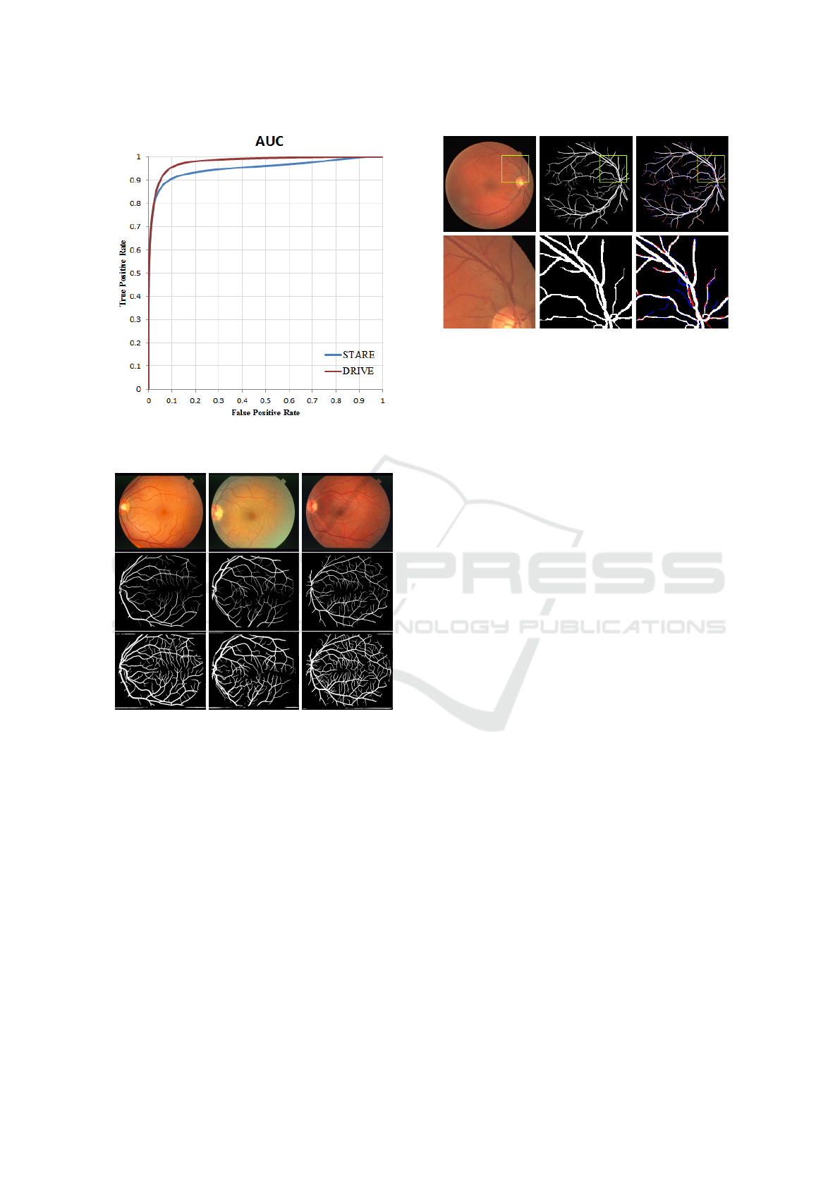
Figure 8: Area Under Curve plots of the DRIVE and
STARE databases.
Figure 9: Segmented images from experiment 4 on the
STARE database. From top to bottom: input image,
ground-truth, segmented images from the large model
trained using a mix of real and synthetic images. It is no-
table that much more small vessels were recognized which
were not segmented by the human expert.
from the STARE results. It is clearly shown that the
proposed method managed to segment the vessels ac-
curately. Figure 8 shows the AUC plot of the pro-
posed method on the STARE database. It is noted
that the proposed model was only trained on DRIVE
data and therefore shows that the applied method
also translates well from DRIVE to the more difficult
STARE data.
Figure 10: An example of the important observation of the
predictions from experiment 4 is shown. From left to right
an image from the DRIVE database, the respective ground-
truth, and the prediction of the combined method are pre-
sented. In the right image, red marks false positive predic-
tions and blue marks true negative predictions.
4.3 Further Observations
An interesting observation of the generated images
is that in some generated images the model extracts
vessels that are not found in the ground-truth images.
Figure 10 shows an example of a segmented image
that contains vessels that are not recognized by the
expert but by the presented network. In Figure 10, the
red color denotes vessels that are in the ground-truth
but the model didn’t detect them as vessels. The blue
color denotes vessels that are extracted by the model
but they are not in the ground-truth.
4.4 Comparison to State-of-the-Art
Methods
To prove the feasibility of using synthetic images for
training, our proposed method is compared against
other deep learning-based methods for retinal blood
vessel segmentation on the DRIVE and STARE
databases. As reported in Table 2 and Table 3, our
method scores the highest sensitivity and AUC com-
paring to the other reported methods.
AUC can be argued to be more relevant since sen-
sitivity, specificity, and accuracy depend on a fixed
threshold. Whereas AUC indicates the accuracy over
all possible thresholds. This indicates that the method
trained on real and synthetic images has the capabil-
ity to detect and segment more vessels than previous
methods. Correspondingly, it also extracts vessel-like
shapes that are not in the ground-truth images. This is
a result of using the synthetic images during training
where the synthetic images cover large different cases
of the vessels tree. From Table 2, it is clearly shown
that the setup of a model with the mixed training data
Synthesizing Fundus Photographies for Training Segmentation Networks
75

Table 2: Comparison of the proposed method trained using mixed images with other CNN-based learning methods on the
DRIVE database.
Method Se Sp Acc AUC
Human observer 0.7598 0.9725 0.9473 -
Zhang et al. (Zhang et al., 2015) - - 0.940 -
Melinscak et al. (Melin
ˇ
s
ˇ
cak et al., 2015) - - 0.9466 0.9749
Liskowski and Krawiec (Liskowski and Krawiec, 2016b) 0.7520 0.9806 0.9515 0.9710
Yao et al. (Yao et al., 2016) 0.7731 0.9603 0.9360 -
Ngo and Han (Ngo and Han, 2017) 0.7464 0.9836 0.9533 0.9752
Soomro et al. (Soomro et al., 2017) 0.746 0.917 0.947 0.8310
Soomro et al. (Soomro et al., 2018) 0.739 0.956 0.948 0.8440
Hu et al. (Hu et al., 2018) 0.7772 0.9793 0.9533 0.9759
Wang et al. (Wang et al., 2019) 0.7986 0.9736 0.9511 0.9740
Feng et al. (Feng et al., 2020) 0.7625 0.9809 0.9528 0.9678
Zou et al. (Zou et al., 2020) 0.7761 0.9792 0.9519 -
Joshua et al. (Joshua et al., 2020) 0.8309 0.9742 0.9615 -
Pedro Costa et al. (Costa et al., 2017b) - - - 0.887 ± 0.004
Our method 0.8334 0.9715 0.9554 0.9784
Table 3: Comparison of the proposed method trained using mixed images with other CNN-based learning methods on the
STARE database.
Method Se Sp Acc AUC
Liskowski and Krawiec (Liskowski and Krawiec, 2016b) 0.8145 0.9866 0.9696 0.988
Soomro et al. (Soomro et al., 2017) 0.748 0.922 0.947 0.853
Soomro et al. (Soomro et al., 2018) 0.748 0.962 0.947 0.855
Hu et al. (Hu et al., 2018) 0.7543 0.9814 0.9632 0.9751
Wang et al. (Wang et al., 2019) 0.7914 0.9722 0.9538 0.9704
Feng et al. (Feng et al., 2020) 0.7709 0.9848 0.9633 0.97
Zou et al. (Zou et al., 2020) 0.7107 0.9754 0.9477 -
Joshua et al. (Joshua et al., 2020) 0.7506 0.9824 0.9658 -
Our method 0.818 0.9705 0.9589 0.9421
Table 4: Quantitative comparison between the proposed
method and approaches for fundus synthesis of Z. (Zhao
et al., 2018) and C. (Costa et al., 2017b). It highlights the
advantage of our method when synthetic images are com-
bined with the data of the DRIVE database.
Data Se Sp AUC
real (ours) 0.7448 0.9796 0.9609
real (Z.) 0.8033 0.9785 -
real (C.) - - 0.887
synthetic (ours) 0.667 0.9858 0.9541
synthetic (Z.) 0.6857 0.9779 -
synthetic (C.) - - 0.841
combined (ours) 0.8334 0.9715 0.9784
combined (Z.) 0.8038 0.9815 -
improves the model performance and outperforms the
usual training techniques on the DRIVE database. Ta-
ble 3 shows the performance of the proposed method
against other methods on the STARE database.
Since the main contribution is the synthesis
pipeline, the proposed method is compared to the
state-of-the-art methods in generating synthetic fun-
dus images by GANs (Costa et al., 2017b), (Zhao
et al., 2018). The results are summarized in Table
4. It can be seen that our approach achieved compa-
rable results with the benefit of a complete adjustable
pipeline for adding characteristics of specific diseases
(see Table 4). The pipeline presented in this work
generates vessel trees which Zhao et al. does not
(Zhao et al., 2018). Additionally, it creates more re-
alistic vessel trees than the GAN approach of Costa
et al. which has recoiling branches and less tiny ves-
sels (Costa et al., 2017b). The recently published ves-
sel tree synthesis approach of Castro et al. was not
evaluated on the task of vessel segmentation and can
therefore not be compared (Castro et al., 2020).
DeLTA 2021 - 2nd International Conference on Deep Learning Theory and Applications
76

5 CONCLUSION
This paper presented a completely new approach to
synthesize retinal fundus photographs and using the
synthetic images for CNN training. In comparison to
other state-of-the-art approaches like the method pre-
sented in (Costa et al., 2017b), the proposed synthe-
sizing method generates a very realistic vessels tree
without unconnected vessels. The final synthesized
image is a realistic image that achieves state-of-the-art
performance in segmentation networks without com-
plex preprocessing and can, therefore, be used to en-
large training sets and solve the problem of lacking
training data. The proposed approach improved the
performance of vessel segmentation as shown quanti-
tatively and qualitatively from the conducted experi-
ments and the comparison against state-of-the-art reti-
nal vessel segmentation.
As future work, we will consider different
databases that are used in retinal vessel segmentation
such as HRF or CHASE DB1 to be synthesized which
includes various disease patterns. The synthesizing
process will be adjustable to generate more realistic
images with different resolutions and generalize the
statistical shapes of different real databases.
Finally, it is stressed that due to the highly ad-
justable pipeline, the generated images are easily use-
able for optic disc segmentation and fovea localiza-
tion tasks.
REFERENCES
Abr
`
amoff, M. D., Garvin, M. K., and Sonka, M. (2010).
Retinal imaging and image analysis. IEEE reviews in
biomedical engineering, 3:169–208.
Al-Diri, B., Hunter, A., and Steel, D. (2009). An ac-
tive contour model for segmenting and measuring reti-
nal vessels. IEEE Transactions on Medical imaging,
28(9):1488–1497.
Bonaldi, L., Menti, E., Ballerini, L., Ruggeri, A., and
Trucco, E. (2016). Automatic generation of synthetic
retinal fundus images: Vascular network. In MIUA,
pages 54–60.
Budai, A., Bock, R., Maier, A., Hornegger, J., and Michel-
son, G. (2013). Robust vessel segmentation in fundus
images. International journal of biomedical imaging,
2013.
Castro, D. L., Valenti, C., and Tegolo, D. (2020). Retinal
image synthesis through the least action principle. In
2020 5th International Conf. on Intelligent Informat-
ics and Biomedical Sciences (ICIIBMS), pages 111–
116. IEEE.
Chaudhuri, S., Chatterjee, S., Katz, N., Nelson, M., and
Goldbaum, M. (1989). Detection of blood vessels in
retinal images using two-dimensional matched filters.
IEEE Transactions on medical imaging, 8(3):263–
269.
Costa, P., Galdran, A., Meyer, M. I., Mendonc¸a, A. M., and
Campilho, A. (2017a). Adversarial synthesis of reti-
nal images from vessel trees. In International Confer-
ence Image Analysis and Recognition, pages 516–523.
Springer.
Costa, P., Galdran, A., Meyer, M. I., Niemeijer, M.,
Abr
`
amoff, M., Mendonc¸a, A. M., and Campilho,
A. (2017b). End-to-end adversarial retinal image
synthesis. IEEE transactions on medical imaging,
37(3):781–791.
Feng, S., Zhuo, Z., Pan, D., and Tian, Q. (2020). Ccnet: A
cross-connected convolutional network for segment-
ing retinal vessels using multi-scale features. Neuro-
computing, 392:268–276.
Fiorini, S., Ballerini, L., Trucco, E., and Ruggeri, A. (2014).
Automatic generation of synthetic retinal fundus im-
ages. In Eurographics Italian Chapter Conference,
pages 41–44.
Guibas, J. T., Virdi, T. S., and Li, P. S. (2017). Synthetic
medical images from dual generative adversarial net-
works. arXiv preprint arXiv:1709.01872.
Hoover, A., Kouznetsova, V., and Goldbaum, M. (2000).
Locating blood vessels in retinal images by piecewise
threshold probing of a matched filter response. IEEE
Transactions on Medical imaging, 19(3):203–210.
Hu, K., Zhang, Z., Niu, X., Zhang, Y., Cao, C., Xiao, F.,
and Gao, X. (2018). Retinal vessel segmentation of
color fundus images using multiscale convolutional
neural network with an improved cross-entropy loss
function. Neurocomputing, 309:179–191.
Ibtehaz, N. and Rahman, M. S. (2020). Multiresunet:
Rethinking the u-net architecture for multimodal
biomedical image segmentation. Neural Networks,
121:74 – 87.
Joshua, A. O., Nelwamondo, F. V., and Mabuza-Hocquet,
G. (2020). Blood vessel segmentation from fundus
images using modified u-net convolutional neural net-
work. Journal of Image and Graphics, 8(1).
Liskowski, P. and Krawiec, K. (2016a). Segmenting reti-
nal blood vessels with deep neural networks. IEEE
transactions on medical imaging, 35(11):2369–2380.
Liskowski, P. and Krawiec, K. (2016b). Segmenting reti-
nal blood vessels with deep neural networks. IEEE
transactions on medical imaging, 35(11):2369–2380.
Mart
´
ınez-P
´
erez, M. E., Hughes, A. D., Stanton, A. V.,
Thom, S. A., Bharath, A. A., and Parker, K. H.
(1999). Retinal blood vessel segmentation by means
of scale-space analysis and region growing. In In-
ternational Conference on Medical Image Comput-
ing and Computer-Assisted Intervention, pages 90–
97. Springer.
Melin
ˇ
s
ˇ
cak, M., Prenta
ˇ
si
´
c, P., and Lon
ˇ
cari
´
c, S. (2015). Reti-
nal vessel segmentation using deep neural networks.
In 10th International Conference on Computer Vision
Theory and Applications (VISAPP 2015).
Ngo, L. and Han, J.-H. (2017). Multi-level deep neural
network for efficient segmentation of blood vessels
Synthesizing Fundus Photographies for Training Segmentation Networks
77

in fundus images. Electronics Letters, 53(16):1096–
1098.
Patton, N., Aslam, T. M., MacGillivray, T., Deary, I. J.,
Dhillon, B., Eikelboom, R. H., Yogesan, K., and Con-
stable, I. J. (2006). Retinal image analysis: concepts,
applications and potential. Progress in retinal and eye
research, 25(1):99–127.
Patzelt, J. (2009). Basics Augenheilkunde. Elsevier, Ur-
ban&FischerVerlag.
Perlin, K. (2002). Improving noise. In Proceedings of the
29th annual conference on Computer graphics and in-
teractive techniques, pages 681–682.
Porter, T. (1984). Compositing digital images. Computer
Graphics Volume18, Number3 July 1984, pages 253–
259.
Soomro, T. A., Afifi, A. J., Gao, J., Hellwich, O., Khan,
M. A., Paul, M., and Zheng, L. (2017). Boosting sen-
sitivity of a retinal vessel segmentation algorithm with
convolutional neural network. In 2017 International
Conference on Digital Image Computing: Techniques
and Applications (DICTA), pages 1–8. IEEE.
Soomro, T. A., Afifi, A. J., Gao, J., Hellwich, O., Paul, M.,
and Zheng, L. (2018). Strided u-net model: Retinal
vessels segmentation using dice loss. In 2018 Dig-
ital Image Computing: Techniques and Applications
(DICTA), pages 1–8. IEEE.
Soomro, T. A., Afifi, A. J., Gao, J., Hellwich, O., Zheng,
L., and Paul, M. (2019a). Strided fully convolutional
neural network for boosting the sensitivity of retinal
blood vessels segmentation. Expert Systems with Ap-
plications, 134:36–52.
Soomro, T. A., Afifi, A. J., Zheng, L., Soomro, S., Gao,
J., Hellwich, O., and Paul, M. (2019b). Deep learn-
ing models for retinal blood vessels segmentation: A
review. IEEE Access, 7:71696–71717.
Staal, J., Abr
`
amoff, M. D., Niemeijer, M., Viergever, M. A.,
and Van Ginneken, B. (2004). Ridge-based vessel seg-
mentation in color images of the retina. IEEE trans-
actions on medical imaging, 23(4):501–509.
Wang, C., Zhao, Z., Ren, Q., Xu, Y., and Yu, Y. (2019).
Dense u-net based on patch-based learning for retinal
vessel segmentation. Entropy, 21(2):168.
Yao, Z., Zhang, Z., and Xu, L.-Q. (2016). Convolu-
tional neural network for retinal blood vessel segmen-
tation. In 2016 9th international symposium on Com-
putational intelligence and design (ISCID), volume 1,
pages 406–409. IEEE.
Zhang, J., Cui, Y., Jiang, W., and Wang, L. (2015). Blood
vessel segmentation of retinal images based on neural
network. In International Conference on Image and
Graphics, pages 11–17. Springer.
Zhao, H., Li, H., Maurer-Stroh, S., and Cheng, L. (2018).
Synthesizing retinal and neuronal images with gener-
ative adversarial nets. Medical image analysis, 49:14–
26.
Zou, B., Dai, Y., He, Q., Zhu, C., Liu, G., Su, Y., and
Tang, R. (2020). Multi-label classification scheme
based on local regression for retinal vessel segmenta-
tion. IEEE/ACM Transactions on Computational Bi-
ology and Bioinformatics.
DeLTA 2021 - 2nd International Conference on Deep Learning Theory and Applications
78
