
Real-time Weapon Detection in Videos
Ahmed Nazeem, Xinzhu Bei, Ruobing Chen and Shreyas Shrivastava
Facebook, U.S.A.
Keywords:
Weapon Detection, Computer Vision Applications, Object Detection, Security.
Abstract:
Real-time weapon detection in video is a challenging object detection task due to the small size of weapons
relative to the image size. Thus, we try to solve the common problem that object detectors deteriorate dramat-
ically as the object becomes smaller. In this manuscript, we aim to detect small-scale non-concealed rifles and
handguns. Our contribution in this paper is (i) proposing a scale-invariant object detection framework that is
particularly effective with small objects classification, (ii) designing anchor scales based on the effective re-
ceptive fields to extend the Single Shot Detection (SSD) model to take an input image of resolution 900*900,
and (iii) proposing customized focal loss with hard-mining. Our proposed model achieved a recall rate of 86%
(94% on rifles and 74% on handguns) with a false positive rate of 0.07% on a self-collected test set of 33K
non-weapon images and 5K weapon images.
1 INTRODUCTION
In recent years, there has been a surge in firearms
violence. Having a weapon detection system that
creates alarms based on live video will be a very
powerful tool to reduce damage. An example use
case is deploying such a weapon detection system
to surveillance cameras. In this use case, the sys-
tem recall can be further improved if more than one
camera is used to capture difference angles and dis-
tances. In the object detection literature, it is widely
accepted that detecting small objects is a challeng-
ing task. The reason off-the-self deep learning de-
tector networks (e.g.,Resnet50 trained on Imagenet,
SSD300 and SSD512) fail in the context of our prob-
lem is the small size of the target objects. In our train-
ing set (collected through lab experiments), more than
50% of the weapon square root area is below 6.5% of
the entire image. This means that for a 300*300 im-
age, 50% of the weapons will have a bounding box
less than 20*20 pixels.
To be able to practically deploy the model, the
number of false alarms should be controlled. In this
paper, we propose a variant of Single Short Detector
(SSD) that is capable of detecting rifles and handguns
at a low false alarm rate. The key contribution of the
paper is proposing an architecture and a loss function
that are capable of attaining a low false positive rate
(0.07%) with high recall (86%) for weapons. The ar-
chitecture is an extension of the SSD model in 3 di-
rections:
1. The input resolution is extended from 300x300
to 900x900 to increase the receptive field of the
bounding boxes.
2. A classification layer is added to classify whether
the entire image contains a weapon or not.
3. A simplified version of feature fusion is utilized
to give bounding boxes more context information
from higher layers.
Additionally, a modified version of focal loss with
hard negative mining was adopted. While localization
accuracy ensures the detector to focus on the crucial
area and improves its recall, the exact localization re-
sults are non-essential to our problem. Hence, while
the localization accuracy is kept in our loss functions,
our metrics shall merely focus on classification. The
rest of the paper is organized as follows: Section 2
reviews the related work. In Section 3, we present
our proposed architecture. Finally, in Section 4, we
present a subset of the experiments we performed to
choose the proposed architecture.
2 RELATED WORK
CNN based object detection methods can be divided
into two-stage detectors and single-stage detectors. In
general, two-stage detectors achieve higher precision
but with lower inference speed. Faster RCNN (Ren
Nazeem, A., Bei, X., Chen, R. and Shrivastava, S.
Real-time Weapon Detection in Videos.
DOI: 10.5220/0010699900003122
In Proceedings of the 11th International Conference on Pattern Recognition Applications and Methods (ICPRAM 2022), pages 497-504
ISBN: 978-989-758-549-4; ISSN: 2184-4313
Copyright
c
2022 by SCITEPRESS – Science and Technology Publications, Lda. All rights reserved
497

et al., 2015) is a major example of two-stage detec-
tors. It generates a series of candidate proposals by
region proposal network (RPN), and then regresses
and classifies these proposals. Its descendants such as
R-FCN (Dai et al., 2016), FPN (Lin et al., 2017a) and
Mask R-CNN (He et al., 2017) are proposed to further
improve the detection accuracy. On the other hand,
the single shot detectors discard the phase of gener-
ating proposals and detect objects in a dense manner
e.g. YOLO (Redmon et al., 2016) and SSD (Liu et al.,
2016). YOLO and SSD adopted a lightweight net-
work as backbone to obtain faster running speed while
in the meantime reach state-of-the-art comparable ac-
curacy. Many advances as in (He et al., 2016) sought
to improve the detection accuracy through adopting
more advanced backbones. On the other hand, in (Lin
et al., 2017b) the authors sought to improve the accu-
racy by adopting focal loss.
Anchor-based object detection methods detect ob-
jects within a set of predetermined anchor boxes gen-
erated at different scales and aspect ratio to cover all
possible object locations in the image. Each anchor
box is associated with a cell in some feature map layer
generated by a convolution network. Anchor-based
methods are used in both single-stage methods and
two-stage methods. It is indicated in (Huang et al.,
2017) that the performance of these detectors deteri-
orates dramatically with small objects. In SSD, lower
features are used to detect small objects, whereas
higher features are used to detect larger objects. How-
ever, the lower features have less semantic informa-
tion. In order to solve this problem, feature fusion
(Lin et al., 2017a) has been proposed for object detec-
tion CNN to improve the precision of smaller objects.
However, this comes with a speed burden.
There have been several directions to improve ac-
curacy for small objects detection. As examples of
SSD extensions: (Lim et al., 2021) proposed to extend
SSD by (i) fusing features from different layers to get
context information while performing the detection,
and (ii) using an attention module for higher features
to improve the detection accuracy. (Jeong et al., 2017)
proposed to jointly (i) concatenate lower features into
higher layers through pooling of lower features, and
(ii) concatenate higher features into lower features
through up-sampling of higher features. (Zhang et al.,
2017) proposed to use an extension of SSD for face
detection. The proposed framework is effective in
detecting small faces. In the proposed framework,
the authors used max-out background labels to re-
duce false positives. Additionally, they proposed to
tile anchors on a wide range of layers to ensure that
all scales of faces have enough features for detection.
In (Sun et al., 2019), the authors proposed to use (i)
weakly-supervised segmentation to assist the object
detector, and (ii) multiple receptive fields blocks as
new convolution predictors for SSD to improve de-
tection accuracy. In (Fu et al., 2017), the authors
(i) combined Resnet101 with SSD, (ii) augmented
SSD+Residual-101 with deconvolution layers to in-
troduce additional large-scale context in object detec-
tion and improve accuracy, especially for small ob-
jects.
(Pang et al., 2019) is an example for two-stage de-
tector extensions for small object accuracy improve-
ments. The authors proposed to use a two-stage detec-
tor of Tiny-Net with a global attention block to reduce
false positives to detect small objects in real-time re-
mote sensing systems. Finally, (Noh et al., 2019) and
(Li et al., 2017) proposed to improve the detection ac-
curacy of small objects using super-resolution.
3 PROPOSED ARCHITECTURE
3.1 A Review of Single Short Detectors
(SSD)
Since our proposed architecture is an extension of
SSD, we start this section by giving a quick intro-
duction for SSD. SSD discretizes the output space
of bounding boxes into a set of default boxes over
different aspect ratios and scales per feature map lo-
cation. At prediction time, the network generates
scores for the presence of each object category in
each default box and produces adjustments to the box
to better match the object shape. Additionally, the
network combines predictions from multiple feature
maps with different resolutions to naturally handle
objects of various sizes. It utilizes VGG16 as a back-
bone with additional convolution layers to create fea-
ture maps of different resolutions. From each of the
feature maps, an additional convolution layer is used
to predict the bounding boxes coordinates and object
classification score. We proposed to extend SSD in 3
directions:
1. Extending the input size from 300x300 to
900x900
2. Adding a classification layer for the entire image
3. Using feature fusion for lower feature maps
The architecture of the proposed model is depicted in
Figure 1.
3.2 Extending SSD300 to SSD900
To extend SSD300 to SSD900, we followed these
three steps:
ICPRAM 2022 - 11th International Conference on Pattern Recognition Applications and Methods
498

Table 1: SSD 900 Feature maps description.
Feature map Min # pixels Max # pixels
size covered by cell covered by cell
57*57 32 63
28*28 64 127
14*14 128 255
7*7 256 511
4*4 512 900
• First, the new features map sizes of the source lay-
ers are indicated in Table 1. Also, the min/max
number of pixels covered by each cell in the fea-
ture map are given in the table. As it can be no-
ticed in the table, the number of source layers was
reduced from 6 to 5. This serves towards an effort
to simplify the model and to reduce the number
of anchor boxes. Additionally, since the goal is
to detect weapons in live videos, the object area
would not consume a big portion of the image.
Hence, we dropped the last source layer.
• Second, due to the huge increase in the number
of the candidate bounding boxes implied by the
increase in resolution, we propose to increase the
stride of the localization and the confidence con-
volution filters applied to the feature layers from 1
to 2. Hence, the feature map sizes are not affected
while the localization accuracy might be slightly
affected. But, as we mentioned in the introductory
section, the classification accuracy is the main fo-
cus of this work.
• Third, since localization is less important,
we used only the following box sizes per
cell: (min,min), (max,max), (min
√
2,min/
√
2),
(min/
√
2,min
√
2) for the bounding boxes of all
feature maps
By using a stride of 2 and using less aspect ratios,
we managed to control the number of bounding boxes
down to 17176 which is just double that of the stan-
dard SSD300 (8732)
3.3 Adding a Classification Layer for
the Entire Image
As shown in Figure 1, an additional classification
layer is created on top of the bounding boxes classi-
fication layers, where the outputs from all the bound-
ing boxes weapon classification results are connected
to this image classification layer after taking the
SoftMax between the classification outputs of each
bounding box. This additional layer helped signifi-
cantly to reduce the false positives.
3.4 Feature Fusion
Motivated by the feature pyramid concept, we imple-
mented a simplified version of the feature fusion em-
ployed in the pyramid. As shown in Figure 2, each of
the source layers is up-sampled using bilinear interpo-
lation, and then concatenated with the previous layer.
Then, a convolution is applied to restore the original
size of the feature map. We tried the conventional
feature pyramids approach in which the fused layer is
up-sampled and concatenated with the previous layer,
but we found that it degraded the performance slightly
and made the model slower. Thus, we resorted to this
simpler version, where each layer gets some context
and semantics information from the successive source
layer.
3.5 Implementation Details
3.5.1 Loss Function
We propose to use three sources of loss: (i) bound-
ing boxes localization loss (L
loc
), (ii) bounding boxes
classification loss (L
Con f Box
), (iii) the entire image
classification loss (L
Con f Image
). As shown in equa-
tions below, the total loss is the weighted sum of
these three sources of loss, where we set the weights
(w
1
,w
2
,w
3
) to (1,10,1) after some hyper-parameter
tuning. For the localization loss, we used the stan-
dard smooth L
1
loss. For the entire image classifi-
cation loss, we used classical cross-entropy. For the
bounding boxes classification loss, we used a mod-
ified version of the focal loss, where the focal loss
is computed separately for the positive boxes and for
the negative boxes. Additionally, the average cross
entropy loss of the hardest negative boxes is added.
Hence, as shown in the equation below, the bounding
boxes classification loss is computed as weighted av-
erage of (i) the average focal loss of positive boxes,
(ii) the average focal loss of negative boxes, and (iii)
the average cross entropy loss of the hardest nega-
tive boxes. The averages are computed per batch, the
weights (w
21
,w
22
,w
23
) are set to (1,1,0.1) after hyper-
parameter tuning and the set of hard negatives HB
−
is
selected as the 10 negative bounding boxes with high-
est confidence score p
i
per batch.
Real-time Weapon Detection in Videos
499
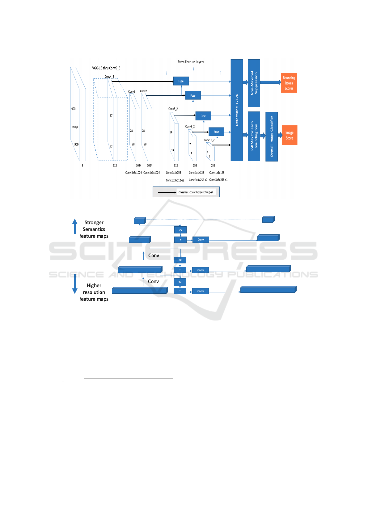
Figure 1: The architecture of the proposed model.
Figure 2: Simplified Feature Fusion.
Loss = w
1
L
loc
+ w
2
L
Con f Box
+ w
3
L
Con f Image
L
loc
= mean
i∈B
+
(
∑
m∈M
smooth
L
1
(l
m
i
−g
m
i
))
L
Con f Box
= −w
21
mean
i∈B
+
((1 −p
i
)
2
log(p
i
)
−w
22
mean
i∈B
−
(p
2
i
log(1 −p
i
))
−w
23
mean
i∈HB
−
(log(1 −p
i
))
L
Con f Image
=
−
∑
j∈I
+
log(q
j
) −
∑
j∈I
−
log(1 −q
j
)
|I
+
|+ |I
−
|
(1)
Where:
• B
+
is the set positive bounding boxes,
• B
−
is the set of negative bounding boxes,
• HB
−
is the set of hard negative bounding boxes,
• I
+
is the set of positive images
• I
−
is the set of negative images
• M is the four bounding boxes coordinates,
• l
m
i
is the m-th predicted coordinate of bounding
box i,
• g
m
i
is the ground truth m-th coordinate of bound-
ing box i,
• p
i
is the confidence score of bounding box i,
• q
j
is the confidence score of image j
3.5.2 Sampling Strategy
Since non-weapon images are much more frequent
than weapon images during the inference time, we
did not seek to oversample the weapon class im-
ages to be more than the non-weapon images class.
Thus, we tried 2 sampling strategies: (weapon =
0.35, non-weapon = 0.65) and (weapon = 0.5 non-
weapon = 0.5). After a few experiments, we con-
ICPRAM 2022 - 11th International Conference on Pattern Recognition Applications and Methods
500

cluded (0.35,0.65) is a better sampling strategy to bal-
ance the recall against the false positive rate.
3.5.3 Data Augmentation
After several experiments, we settled on applying the
following techniques to the training set (i) rotation
with probability 0.5 with an angle between 0 and 90,
(ii) translation with probability 0.5 with 50% magni-
tude, (iii) horizontal mirroring with probability of 0.5,
and (iv) we ruled out scaling as it did not help.
Some tips for maintaining numerical stability with
custom loss functions:
• Make sure to add Epsilon whenever we take Soft-
Max
• Set a maximum and a minimum for the loss and
the gradients vectors
• Apply some smoothing mechanism for the final
loss magnitude after each iteration to avoid spurs
4 EXPERIMENTS
4.1 Data Collection
To build our initial model, we collected about 55K
images (42K non weapons-13K weapons). Weapons
were carried at different angles, distances, and speed.
Multiple lab cameras were used with different alti-
tude, angle and resolution. Examples of hard nega-
tive objects are umbrellas, cell phones, sticks, badges
and brooms. Then, we performed a wide range of ex-
periments to select the best model architecture. After
we selected the model architecture and built our ini-
tial model, we proceeded to improve the model per-
formance by ingesting more data. Inspired by active
learning, we sought to collect hard examples as fol-
lows:
• To collect hard positives examples, we ran lab
experiments against our latest model. Then, we
annotated and added the instances whose scores
were slightly below the classification threshold.
Our rationale was that these examples whose
scores are not very far from the classification
threshold are false negatives that the model can
improve on, whereas those with very small scores
might have an adverse effect on the false positive
rate. Additionally, for low score false negatives,
we found that it was usually hard for a neutral an-
notator to decide whether they contain weapons
or not because of the distance, the angle or the oc-
clusion.
• In a similar manner, to collect hard negative ex-
amples, we ran lab experiments against our latest
model. Then, we added all the instances with rel-
atively high scores to our data set.
The data collection procedure is iterative. As we
collect some hard examples and we update our train
and test sets, we retrain our model with the addi-
tional data. Then, we use the updated model for the
next round of data collection. We ended up collect-
ing about 125K images of which: 10% validation,
25% testing, 65% training. 15% of the image were
weapons and 85% were non-weapons. For the nega-
tive photos, we had 15% easy negatives and 85% hard
negatives.
4.2 Ablation Study
In this section, we compare the metrics drawn from
training 6 different architectures using the same
dataset. The training set contains 74K non-weapon
images and 13K weapon images, of which 7.4K non-
weapon images and 1.3K weapon images are used
for validation. The evaluation set contains 33K non-
weapon images and 5K weapon images. The reported
architectures are:
1. Standard SSD 300 + standard SSD loss
2. SSD 300 + feature fusion + custom focal loss
3. SSD 512 + feature fusion + custom focal loss
4. SSD 900 + feature fusion + standard SSD loss
5. SSD 900 + custom focal loss
6. SSD 900 + feature fusion + custom focal loss
Since the negative class dominates the positive class,
the metrics recommended by business were F0.5
score, false positive rate at 80% recall, and recall rate
at 0.1% false positive rate. These metrics along with
fpr and recall at threshold of 0.5 are listed in Table 2.
By looking at Table 2, we can see the following:
• The recall for the basic SSD300 is very low (52%
at threshold=0.5).
• Comparing (2) to (1): Adding feature fusion and
custom focal loss to SSD 300 resulted in a huge
boost to recall (from 52% to 92%) on the ex-
pense of a higher false positive rate (from 0.2% to
4.98%). F0.5 score stayed almost the same with
some improvements in the threshold range [0.55-
0.75].
• Comparing (3) to (2): Increasing the resolution
from 300 to 512 improved the recall (from 92%
to 98%) but that came with a slight increase in
false positive rate (from 4.98% to 5.74%). F0.5
Real-time Weapon Detection in Videos
501

score stayed almost the same with some improve-
ments about threshold of 0.65 due to higher scores
of true positives.
• Comparing (6) to (3): Increasing the resolution
from 512 to 900 led to a huge decrease in false
positive rate (from 5.74% to 0.11%). On the other
hand, it decreased the recall at threshold less than
0.7 but improved it at higher thresholds. Our in-
tuition is that for the model to take down on fpr, it
had to go slightly worse at the recall of hard posi-
tives that are not easily distinguishable from hard
negatives. We sampled some of those missed hard
positives and we found that it is hard for a neutral
human annotator to classify them. On the other
hand, the model was able to get better at the recall
of easier positives.
• Comparing (6) to (4): Custom focal loss at a reso-
lution of 900 led to a huge increase in recall (64%
to 89%) and was neutral on fpr.
• Comparing (6) to (5): Feature fusion at a reso-
lution of 900 led to a significant decrease in fpr
(0.64% to 0.11%) and was neutral on recall.
In Figure 3, we present more statistics for architecture
number 6. We can summarize it by saying that at the
chosen operating point of 0.6 classification threshold,
the model has:
• 86% Recall
• 94% Recall for rifles
• 74% Recall for guns
• 0.07% False positive rate
• 99.47% Precision
• 98% accuracy
4.3 Training Details
1. 150 epochs.
2. Step LR scheduler with gamma of 0.5 every 30
epochs
3. SGD optimization algorithm with weight decay
0.00001, momentum 0.9, 0.001 learning rate
4. 32 GPUs where the batch size on each GPU is 4
images.
5. All layers are optimized.
6. The total training time varied from 40 hours for
SSD300 to 60 hours for SSD900.
7. In the recurrent training, when new data is added,
the model trains for 10 epochs starting from the
latest version.
4.4 Inference Considerations
• At inference time, the overall image classification
score is ignored, and the bounding box score is
used. While the overall image classification loss
helps as an additional source of loss when com-
bined with bounding box loss, using the overall
image score as the major decision criterion for in-
ference leads to overfitting as it is less location-
invariant compared to bounding box score.
• The model was built using PyTorch, then it was
exported via Torchscript to run in C++ environ-
ment.
• The frame rate per seconds (fps) for architecture
(2) on CPU is about 4.5 fps, whereas the fps for
architecture (6) is about 0.45 fps. Thus, for practi-
cal considerations, we propose to use a two stage
cascaded models as follows:
1. Stage 1: use architecture (2) characterized by
high recall (92%) and relatively high fpr (5%).
This will filter out more than 95% of image
frames.
2. Stage 2: for those frames classified as positive
by Stage 1, use architecture (6), characterized
by high recall (86%) and very low fpr (0.07%),
to confirm the final decision if the frame con-
tains a weapon or not.
3. The expected system fps will be equal to
0.05*0.5+0.95*5 = 4.34 fps which is very close
to SSD300 throughput but with a much higher
recall and fpr. The 2-stage model has a recall of
79% and an fpr of 0.04%.
4.5 Explored Ideas that Did Not
Produce Improvements
1. Standard Faster-RCNN resulted in an extremely
high false positive rate.
2. Decrease the number of output neurons per
bounding box to 1 instead of 2.
3. Freezing the base or extra layers. This led to a
sharp degradation in performance.
4. Cascaded bounding boxes classifiers. The idea is
borrowed from Viola and Jones where for each
bounding box, we have a set of cascaded classi-
fiers.
5. Auxiliary Segmentation. Similar to (Sun et al.,
2019).
6. Image tiling: Divide each image into 6 overlap-
ping grids and perform the training and the infer-
ence on the grids.
ICPRAM 2022 - 11th International Conference on Pattern Recognition Applications and Methods
502
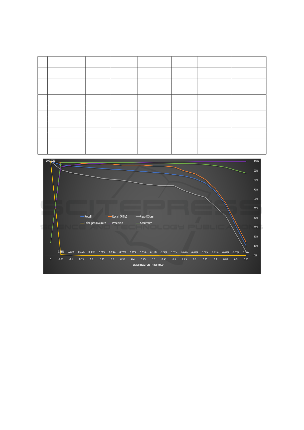
Table 2: Candidate architectures metrics.
Id Architecture Max F0.5 FPR at FPR at Recall at Recall at Inference time
Score 80% recall threshold =0.5 0.1% FPR threshold =0.5
1 Standard SSD 0.893 1.17% 0.2% 38% 52% 0.2 sec
300
2 SSD 300 + 0.897 1.11% 4.98% 27% 92% 0.22 sec
feature fusion +
custom focal loss
3 SSD 512 + 0.897 1.75% 5.74% 19% 98% 0.7 sec
feature fusion +
custom focal loss
4 SSD 900 + 0.952 0.23% 0.09% 64% 64% 2.2 sec
feature fusion +
standard loss
5 SSD 900 + 0.941 0.33% 0.64% 46% 88% 1.9 sec
custom focal loss
6 SSD 900 + 0.97 0.05% 0.11% 88% 89% 2.2 sec
feature fusion +
custom focal loss
Figure 3: Metrics of architecture #6.
7. Bounding boxes max-out: Similar to (Zhang
et al., 2017).
5 CONCLUSION
This paper introduces an object detection framework
that is particularly effective with small object binary
classification. We extend the SSD to take an input im-
age of resolution 900 to improve false positive rate.
Additionally, we propose a new loss function that is
particularly effective in handling the class imbalance,
and in reducing false positives. In the future, we are
planning to work on (i)compressing the network for
faster inference time, (ii) introducing more types of
weapons, and (iii) introducing real video data (not
collected from lab experiments).
REFERENCES
Dai, J., Li, Y., He, K., and Sun, J. (2016). R-fcn: Object de-
tection via region-based fully convolutional networks.
In Advances in neural information processing sys-
tems, pages 379–387.
Fu, C.-Y., Liu, W., Ranga, A., Tyagi, A., and Berg, A. C.
(2017). Dssd: Deconvolutional single shot detector.
arXiv preprint arXiv:1701.06659.
Real-time Weapon Detection in Videos
503

He, K., Gkioxari, G., Doll
´
ar, P., and Girshick, R. (2017).
Mask r-cnn. In Proceedings of the IEEE international
conference on computer vision, pages 2961–2969.
He, K., Zhang, X., Ren, S., and Sun, J. (2016). Deep resid-
ual learning for image recognition. In Proceedings of
the IEEE conference on computer vision and pattern
recognition, pages 770–778.
Huang, J., Rathod, V., Sun, C., Zhu, M., Korattikara, A.,
Fathi, A., Fischer, I., Wojna, Z., Song, Y., Guadar-
rama, S., et al. (2017). Speed/accuracy trade-offs for
modern convolutional object detectors. In Proceed-
ings of the IEEE conference on computer vision and
pattern recognition, pages 7310–7311.
Jeong, J., Park, H., and Kwak, N. (2017). Enhancement
of ssd by concatenating feature maps for object detec-
tion. arXiv preprint arXiv:1705.09587.
Li, J., Liang, X., Wei, Y., Xu, T., Feng, J., and Yan, S.
(2017). Perceptual generative adversarial networks for
small object detection. In Proceedings of the IEEE
conference on computer vision and pattern recogni-
tion, pages 1222–1230.
Lim, J.-S., Astrid, M., Yoon, H.-J., and Lee, S.-I. (2021).
Small object detection using context and attention.
In 2021 International Conference on Artificial Intel-
ligence in Information and Communication (ICAIIC),
pages 181–186. IEEE.
Lin, T.-Y., Doll
´
ar, P., Girshick, R., He, K., Hariharan, B.,
and Belongie, S. (2017a). Feature pyramid networks
for object detection. In Proceedings of the IEEE con-
ference on computer vision and pattern recognition,
pages 2117–2125.
Lin, T.-Y., Goyal, P., Girshick, R., He, K., and Doll
´
ar, P.
(2017b). Focal loss for dense object detection. In
Proceedings of the IEEE international conference on
computer vision, pages 2980–2988.
Liu, W., Anguelov, D., Erhan, D., Szegedy, C., Reed, S.,
Fu, C.-Y., and Berg, A. C. (2016). Ssd: Single shot
multibox detector. In European conference on com-
puter vision, pages 21–37. Springer.
Noh, J., Bae, W., Lee, W., Seo, J., and Kim, G. (2019). Bet-
ter to follow, follow to be better: Towards precise su-
pervision of feature super-resolution for small object
detection. In Proceedings of the IEEE/CVF Interna-
tional Conference on Computer Vision, pages 9725–
9734.
Pang, J., Li, C., Shi, J., Xu, Z., and Feng, H. (2019). R2-
cnn: Fast tiny object detection in large-scale remote
sensing images. IEEE Transactions on Geoscience
and Remote Sensing, 57(8):5512–5524.
Redmon, J., Divvala, S., Girshick, R., and Farhadi, A.
(2016). You only look once: Unified, real-time object
detection. In Proceedings of the IEEE conference on
computer vision and pattern recognition, pages 779–
788.
Ren, S., He, K., Girshick, R., and Sun, J. (2015). Faster
r-cnn: Towards real-time object detection with region
proposal networks. Advances in neural information
processing systems, 28:91–99.
Sun, S., Yin, Y., Wang, X., Xu, D., Zhao, Y., and
Shen, H. (2019). Multiple receptive fields and
small-object-focusing weakly-supervised segmenta-
tion network for fast object detection. arXiv preprint
arXiv:1904.12619.
Zhang, S., Zhu, X., Lei, Z., Shi, H., Wang, X., and Li, S. Z.
(2017). S3fd: Single shot scale-invariant face detector.
In Proceedings of the IEEE international conference
on computer vision, pages 192–201.
ICPRAM 2022 - 11th International Conference on Pattern Recognition Applications and Methods
504
