Towards a Robust, Distributed and Decentralised Smart Energy

Management of Microgrids

Sandra Garcia-Rodriguez

and Hassan A. Sleiman

Universit

e Paris-Saclay, CEA, List, F-91120 Palaiseau, France

Keywords:

Microgrids, Robust Decentralised Optimisation, Multi-Agent System, Evolutionary Computation.

Abstract:

Modern energy systems comprise different entities that interact to allow an intelligent production, distribution,

and consumption of energy. They need efﬁcient and distributed demand-response management mechanisms

to ﬁnd optimised conﬁgurations of parameters of the grid components. When working with time schedules,

optimisation algorithms used for this purpose usually rely on forecasts. However, forecasts bring uncertainty,

which is rarely considered in optimisation. This work presents a robust and decentralised optimisation ap-

proach that deals also with such uncertainty by searching for optimal power schedule solutions, which are

also reliable in unexpected circumstances. Based on message passing, our approach uses meta-heuristics for

performing local optimisations. The implementation and validation of our proposal was conducted by means

of a distributed multi-agent system, where the obtained results have shown the efﬁciency of our approach.

1 INTRODUCTION

Smart grids became one of the solutions to deal with

climate change and the continually increasing de-

mand for energy (Tuballa and Abundo, 2016). It is

an intelligent electrical grid with a distributed energy

generation, storage, integrating of customer power

supply and renewable energy. It is intended to en-

hance the effectiveness and efﬁciency of power deliv-

ery by using intelligent algorithms to manage the pro-

duction, distribution, and consumption of electricity.

The successful implementations of smart grids have

increased the research interest in this ﬁeld.

This article focuses on a part of smart grids, called

microgrids. Microgrids are networked groups of dis-

tributed energy resources, such as solar panels or

wind turbines, located at the distribution network

side, and able to provide energy to small geographical

areas (Saad et al., 2012). It connects consumers (a.k.a

prosumers), which are small-scale co-providers of en-

ergy, and allows local electricity interchange among

them. Such interchange reduces their dependence

on the public grid, placing the generation of elec-

tricity near the end-users. Efﬁcient demand-response

management mechanisms allows users to be energy-

efﬁcient in the long term (Mesaric et al., 2017).

https://orcid.org/0000-0002-5352-2510

https://orcid.org/0000-0002-0018-0027

Efﬁcient demand-response management mecha-

nisms are essential for microgrids since they pursue to

ﬁnd the best conﬁguration parameters of the compo-

nents for an optimised grid performance (Colak et al.,

2016). Such mechanisms manage the grid and try to

achieve an optimised performance for a given objec-

tive(s) such as reducing the bill, avoid power peaks

and/or energy losses, without violating the constraints

imposed by the grid deﬁnition. These decisions are

considered as optimisation problems, and are the fo-

cus of many recent studies (Gomez-Sanz et al., 2014).

In practice, the grid conﬁguration parameters vary

from the time schedules (for a given time horizon),

to the real-time parameters (Gamarra and Guerrero,

2015). Unfortunately, the complexity arises with the

number of variables to be optimised such as the time

setups for self-controlled resources of the grid (Mo-

hamed and Koivo, 2007).

To work with scheduled conﬁgurations, optimis-

ers usually rely on forecasts instead of real-time se-

tups. Forecasts provide an estimation on what may

occur in the near future, allowing to plan the strat-

egy in advance. Currently, many types of forecasts

can be considered in a microgrid optimisation prob-

lem: some of them are related to power consump-

tion/generation such as consumption schedules, bat-

tery levels, production curve; others are related to

weather prediction, such as solar radiation and wind

speed. However, since forecasts are not 100% ac-

Garcia-Rodriguez, S. and Sleiman, H.

Towards a Robust, Distributed and Decentralised Smart Energy Management of Microgrids.

DOI: 10.5220/0010748900003116

In Proceedings of the 14th International Conference on Agents and Artiﬁcial Intelligence (ICAART 2022) - Volume 1, pages 15-25

ISBN: 978-989-758-547-0; ISSN: 2184-433X

curate (Mahat et al., 2013), the observed parameters

may vary from the forecasted ones, which leads to

unexpected situations. In this case, the optimised

solutions (based on the non-accurate forecasts) are

more likely to lie far from the optimal ones (Garc

ıa

et al., 2012), which may provoke looses in money,

resources, and/or time (Liang and Zhuang, 2014).

Therefore, forecasting reliability is a key factor in op-

timisation solutions (Moreno et al., 2017).

In this paper, we present a robust and decen-

tralised optimisation algorithm implemented in a dis-

tributed manner for ﬁnding the best setup conﬁgura-

tion for the devices in a microgrid. We refer to robust-

ness as the capacity of the approach to provide stable

solutions with a performance that does not drop when

unexpected scenarios are faced. Our proposal is based

on the adaptation of the message passing algorithm

proposed by Kraning et al. (Kraning et al., 2014),

where optimisation is split in less complex problems

that are locally solved in different nodes of the grid.

The global optimisation is achieved by means of a

negotiation protocol amongst all of the grid nodes.

Local optimisations are performed using evolution-

ary computation (Zhang et al., 2011), which is con-

sidered an adequate approach for this kind of prob-

lems (Moghaddam et al., 2011; Ramaswamy and De-

coninck, 2012). For instance, metaheuristics as “Par-

ticle Swarm Optimisation” (Chen and Yu, 2005) and

SPEA2 (Zitzler et al., 2001) are adapted to our prob-

lem. Furthermore, in order to deal with the reliabil-

ity of forecasts, we consider the robustness concept

by extending the decentralised optimisation algorithm

with a robust approach, which allows handling the un-

certainty in forecasts within the optimisation process.

Our proposal was implemented by means of a

distributed multi-agent system (Al-Hinai and Alh-

elou, 2021), a technology that has been proven to be

very suitable for microgrid solutions (Farhangi, 2010;

Amin and Wollenberg, 2005). A sliding window over

different year-observations (extracted from real data

sets) was used to carry out our validation tests. Ac-

cording to the results, our algorithm provides effec-

tive solutions by considering uncertainty in its param-

eters. Comparing the optimised schedules obtained

from forecasted parameters to the equivalent real-time

ones, we can see that costs are reduced up to 60% in

some of the tested scenarios.

This paper is organized as follows: Section 2 re-

views the state of the art about distributed optimisa-

tion algorithms for microgrids; Section 3 presents the

algorithm in which the proposed solution is based;

Section 4 details our contribution, whereas Section 5

reports on the validation results. Finally Section 6

concludes our work and discusses the future lines.

2 RELATED WORK

Demand response algorithms emerged in the 1970’s,

but have experienced a renaissance by the appearance

of microgrids (Mihaylov et al., 2019). These algo-

rithms try to optimise the schedules of the control-

lable loads to satisfy the grid objectives, such as val-

ley ﬁlling and peak shaving to mention a few.

The literature reports on many optimisation al-

gorithms for microgrids, which aim at reducing the

energy imbalance and at covering the demand and

supply gap. Some of these approaches are based on

predictions only, whereas others consider the unre-

liability of predictions, aka uncertainty. One of the

main sources of uncertainty in smart grids is the in-

tegration of stochastic renewable energy sources and

the introduction of new energy intensive appliances,

which make it increasingly difﬁcult to ﬁnd an opti-

mised planning of resources in the smart grid (Decon-

inck et al., 2008; Veldman et al., 2013).

The authors in (Haring et al., 2016) developed and

compared three different schemas for optimising the

energy market, involving the customers and focusing

on the trade-off among privacy, resource exploitation

and the reward earned. The ﬁrst schema provided a

centralised optimisation in which the user informa-

tion is shared with the system operator; the second

applied a centralised optimisation, based on an ag-

gregator, with whom the user partially shares cost in-

formation; and the third schema proposed a decen-

tralised schema, in which the prosumers exchanged

energy among each other without revealing their cost

information. Prediction is used in the second schema,

but without considering uncertainty.

Alternating Direction Method of Multipliers

(ADMM (Boyd et al., 2011)) was used in (Rivera

et al., 2017) and (Diekerhof et al., 2014). (Rivera

et al., 2017) proposed a scalable distributed convex

optimisation framework for electrical vehicle aggre-

gators, and covered local and global objectives and

constraints. It is intended to resolve valley ﬁlling and

minimising charging costs by providing optimised

charging plans. It focused on demonstrating the pos-

sibility of integrating electrical vehicles in the grid

and on the scalability of the framework, but it does

no tackle the uncertainty. (Diekerhof et al., 2014)

proposed a distributed optimisation system for intel-

ligently controlling electrical heat pumps at district

level, based on an ADMM, where the local objec-

tives of each participant are considered achieving the

global objectives. The authors in (Diekerhof et al.,

2016) showed the advantages and disadvantages of

distributed optimisations and proposed a particular

usage of ADMM for scheduling electro-thermal heat-

ICAART 2022 - 14th International Conference on Agents and Artiﬁcial Intelligence

ing units. Dantzig-Wolfe decomposition (Dantzig and

Wolfe, 1960) was used by (McNamara and McLoone,

2015), who proposed a hierarchical demand-response

algorithm. The objective of this approach was to peak

minimisation and achieve both: the device and the

customer objectives. Furthermore, it tried to min-

imise the communication overheads and to improve

the quality of service by improving the response time

for the devices that need their energy as soon as pos-

sible. This work does not consider considering uncer-

tainty either.

The following proposals focused on decentralised

frameworks without including uncertainty (de Ce-

rio Mendaza et al., 2016; Meyn et al., 2015): (i)

(de Cerio Mendaza et al., 2016) proposed a hierarchi-

cal and decentralised framework that is intended for

controlling the demand-response in low voltage net-

works, where the system operator plays the aggrega-

tor role for trading energy demand ﬂexibility and for

ensuring reliability and security. Since the framework

only focused on the demand side, just loads were con-

sidered. The authors modelled the heat pumps sys-

tems to respond to demand aggregations, which is

used in their hierarchical structure; (ii) (Meyn et al.,

2015) proposed a decentralised decision making ar-

chitecture for automated demand response that can be

used for maintaining demand-supply balance. The au-

thors provided a solution based on a randomised con-

trol strategy (using a Markovian Decision Process)

to obtain an aggregate model for a large number of

loads. Then, a so-called linear time-invariant sys-

tem approximation of the aggregate nonlinear model

is used for control design at grid level.

However, there are some proposals in the liter-

ature which do consider different kinds of uncer-

tainty in their optimisation algorithms (Moreno et al.,

2017). The authors in (Diekerhof et al., 2014) ap-

plied ADMM in a hierarchical architecture, and com-

bined it with robust optimisation and model predictive

control to handle uncertainty in heat pump schedul-

ing (Diekerhof et al., 2017). (Tajalli et al., 2021)

presented an approach for uncertainty aware manage-

ment of smart grids by using cloud based LSTM inter-

val prediction. (Chakraborty and Okabe, 2016) used

probabilistic programming approach that utilises a

Bayesian Markov Chain Monte Carlo (MCMC) sam-

pling method to create energy based balanced groups.

This allows grouping similar customers whose aggre-

gated demand has higher predictability. To face en-

ergy imbalance problem and cost reduction, the au-

thors proposed a multi-objective optimisation based

on ADMM for scheduling electrical storage units,

considering the demand uncertainty. (Zhang and Gi-

annakis, 2016) formulates a stochastic optimisation

problem based on ADMM also considering uncer-

tainty for market clearance. (Zhang et al., 2017)

contributes with a distributed robust optimiser, con-

sidering uncertainty, which uses the aggregation of

loads for service provision. Finally, (Dehghanpour

et al., 2017) also showed a hierarchical multi-agent

system framework for modelling demand response

of air conditioning loads with a day-ahead planning.

Such framework uses machine learning to model the

behaviours of agents at different levels of the frame-

work. The authors compared linear modelling and

ANN-based modelling to check the learning model

that provides more cut in the consumption cost and

maximise the beneﬁts of the retailer.

As for the technologies used in the implementa-

tion of the algorithms that control microgrids, multi-

agent systems (MAS) technologies are considered

as potential solutions to the power industry pro-

viding ﬂexible, extensible, and fault-tolerant solu-

tions (McArthur et al., 2007a; McArthur et al.,

2007b). They enable the implementation of large and

complex distributed applications by allowing the de-

velopment of autonomous control agents that are able

to coordinate in a cooperative and fault-tolerant en-

vironment (Al-Hinai and Alhelou, 2021). The dis-

tribution and communication characteristics of MASs

are attracting the attention in smart grids due to their

ability to unlock their potentials (Farhangi, 2010); i.e,

the autonomy of agents are adequate for the smart

devices, whereas the grid energy consumption and

production optimisation, usually performed by nego-

tiations, can be easily implemented using the agents

communication mechanisms and protocols.

Our system allows scheduling electrical units by

using the decentralised and distributed optimisation

algorithm (Kraning et al., 2014) that relies in local op-

timisations. Furthermore, it considers uncertainty in

the optimisation so that solutions become more stable

against not accurate predictions. Unlike the papers

mentioned in this section, our robust mechanism can

be adapted to any optimisation algorithm since it deals

with robustness within the cost function. Moreover

we introduce an uncertainty estimation which is only

calculated from forecasts and can be applied to any

device whose forecast values are considered for the

optimisation. This means that we do not need to cre-

ate a new robustness measure for each device model

since uncertainty is speciﬁcally computed for each de-

vice according to its historical observations and fore-

casts.

Towards a Robust, Distributed and Decentralised Smart Energy Management of Microgrids

3 BACKGROUND

Our proposal is based on a fully decentralised method

for dynamic network energy management that uses

message passing between entities (Kraning et al.,

2014).This work models a cooperation network com-

posed by two types of nodes, namely: the devices and

the nets. The devices (i.e. generators, ﬁxed loads,

deferrable loads, alternate direct current transmission

lines, storage units, etc.) have their own constraints

and objectives. Devices are connected through ter-

minals to each other by means of a net (i.e. bus),

which also has its own objectives and constraints. In

the same way, nets are connected through double ter-

minal devices, such as transmission lines. A terminal

is a connection point or a link between the net and the

device.

The goal is to minimise the total network objec-

tive subject to device and net constraints over a time

horizon. For this, (Kraning et al., 2014) method re-

lies on the alternating direction method of multipliers

(ADMM), which is an algorithm that solves convex

optimisation problems by breaking them into smaller

pieces so that they will be then easier to handle (Boyd

et al., 2011).

By relaxing the equations (see (Kraning et al.,

2014) for details), the result is an iterative algorithm

that runs until the convergence criteria is satisﬁed.

Therefore at each iteration k the following operations

are performed in parallel:

• Every device d computes, for each termi-

nal, a new proximal power schedule p

(1),..., p

(H)] ∈ R

that minimises a local ob-

jective function.

The problem is formulated as shown in Equa-

tion 1:

minimize

) +

||p

− (p

− p

+ u

)||

subject to constraints

(1)

Formally, H is the number of time periods to

schedule (time horizon) and ρ is a scaling param-

eter. p

is the current power schedule of device

d computed in previous iteration, and p

the av-

erage of p

of each terminal (in case of just one

terminal devices p

= p

In the same way, u

= [u

(1),...,u

(H)] ∈ R

the scale price received from the net in the previ-

ous iteration. f

) = c

) represents the cost

function c

) of applying p

to d. Note that

each kind of device has a speciﬁc c

) formula.

However, solving the equation 1 also requires

to satisfy the constraints imposed by the device

model. Some of them are already considered

within the cost function c

) of the device,

whereas local optimisers deal with the rest (see

section 5.1 for more details).

Finally, the device sends a message with p

to its

corresponding neighbour net(s). In case of two

terminal devices, the previous operations are re-

peated to compute p

for each net terminal.

• Every net n updates its scale price as u

= u

+ p

where p

is the average of all p

received from

their devices. Finally, u

is sent to all its linked

devices.

The authors showed that their approach converges

to a solution when the objectives and constraints of

the devices are convex. Such solution is decentralised

solution and needs no global coordination other than

synchronizing iterations; the problems to be solved

by each device can be locally solved efﬁciently and

in parallel according to the authors (Kraning et al.,

2014).

4 ROBUST DECENTRALISED

POWER SCHEDULING

OPTIMISER

This paper proposes a novel robust and decentralised

approach algorithm for solving power scheduling

problems in microgrids. Relying in the decentralised

method for dynamic network energy management

presented in section 3, we developed a robust adapta-

tion to deal with uncertainty of parameters during the

optimisation process. Our approach is implemented

within a distributed multi-agent system which allows

solving it in parallel.

In order to calculate the best power schedules

for each time period, the optimization algorithm

needs to know, in advance for these periods, the

power load curve for those devices whose regimes

cannot be controlled and the power curves estima-

tions (as maximum power generation, expected con-

sumption...) in case of self-controlled devices. Un-

fortunately, those forecasts are estimations about the

future which cannot be certain. Big deviations from

real conditions may lead to inefﬁcient power sched-

ules that can provoke several losses as money, energy,

etc. A main contribution of this paper is the consider-

ation of such forecasts uncertainty to guide the opti-

misation process. We developed a robust mechanism

which, adapted within the cost function of those de-

vices subject to uncertainty, increases the reliability of

ICAART 2022 - 14th International Conference on Agents and Artiﬁcial Intelligence

solutions by remaining more stable when unexpected

situations are faced.

The following Section 4.1 shows the implemen-

tation of the proposed approach whereas section 4.2

describes its robust mechanism.

4.1 Implementation

Our algorithm is implemented within a distributed

Multi-Agent System, which is based on the re-usable

architecture already introduced in (Garcia-Rodriguez

et al., 2016). Each device/net composing the micro-

grid is managed by an agent in our system which is in

charge of running a local optimisation and exchang-

ing messages with its neighbour agents. Since decen-

tralization allows distributed implementation, prob-

lem complexity is reduced by splitting computation

load in different nodes. Moreover, unlike centralised

systems which depend on a central node, our ap-

proach achieves smartness by the negotiation of all of

them. This way the probability of facing bottle neck

situations is signiﬁcantly reduced.

Evolutionary computation (Zhang et al., 2011) is

selected for solving the local optimisation function of

equation 1. The use of this kind of algorithms is recur-

rent in the literature since they are proved to be good

approaches to solve microgrid problems (Sanseverino

et al., 2011). For instance, their ﬂexibility allows to

handle most of the hard constraints in the optimisation

process (as the ones of transmission lines presented in

section 5.1). Moreover, their operators can be easily

modiﬁed to improve the algorithm performance in the

speciﬁc problem to solve. Our approach counts with

the following meta-heuristics:

• Mono-objective optimisers (problems with just

one objective function): naturally inspired algo-

rithms as particle swarm optimisation PSO (Chen

and Yu, 2005), differential evolution (Storn and

Price, 1997) or CMAES (Auger et al., 2004).

• Multi-objective optimisers (two or more objec-

tive functions): evolutionary algorithms such as

NSGA-II (Deb et al., 2002) or SPEA2 (Zitzler

et al., 2001).

Thanks to the architecture of our frame-

work (Garcia-Rodriguez et al., 2016), algorithms can

be easily added/replaced. This allowed us choosing

the best one for each local cost function.

4.2 Dealing with Uncertainty

The robust method presented here is applicable when

device forecasts (that are subject to uncertainty) are

used to optimise the microgrid power schedules.

Based on historical forecasts and observations, our

approach guides the optimisation process towards so-

lutions that shall remain stable even when forecasts

result to be very inaccurate. The main strength of this

approach lies in the use of a penalty factor, w

used to penalise the device cost function f

) of

Equation 1. The fact of placing such penalty within

the device cost function makes it easily adaptable to

any other optimisation algorithm. The penalty fac-

tor is computed for each device d according to its

proposed power schedule p

and its historical set of

observations-forecasts.

Therefore, for any device d whose forecasts are

used for optimising its power schedule over a time

horizon H, we can apply the robust improvement that

works as a two-phase algorithm.

4.2.1 First Phase

It is run ofﬂine and before the optimisation process

starts. Relying in the set of historical pairs forecasted-

observed parameters of the device, it computes three

values that will be used in the second phase:

• O f

: proportion of all observed values of d that

were greater than their forecasts in the historical

observations-forecasts set. O f

∈ [0, 1].

• Fo

: proportion of all observed values of d that

were smaller than their forecasts in the historical

observations-forecasts set. Fo

∈ [0, 1].

• UF

: performance of the forecast algorithm used

for computing the forecast parameters of the de-

vice. Its value is calculated in Equation 2 by

measuring the absolute proportional deviation be-

tween the historical real observations and their

corresponding forecasts over the time periods

[1...H] to be optimised:

max

∗ H

∑

t=1

| f p

(t) − op

(t)| (2)

where H is the time horizon; f p

(t) is the fore-

casted parameter and op

(t) the observed param-

eter, both for time periods t ∈ [1...H]; and max

the maximum observed value registered in device

4.2.2 Second Phase

It is called each time the optimisation algorithm eval-

uates the cost function of Equation 1. The steps fol-

lowed in this phase (see Algorithm 1) give an eval-

uation of the risk and negative impact of applying

the power schedule p

to device d. Such evaluation

Towards a Robust, Distributed and Decentralised Smart Energy Management of Microgrids

(penalty factor) is used to guide the optimisation to-

wards robust solutions.

For each time period (line 2), algorithm 1 ﬁrst es-

timates the possible deviations of the proposed power

schedule p

(line 9). Then, considering the im-

port/export prices and constraints, it computes the

corresponding cost of those deviations from apply-

ing the proposed power schedule p

to a full power

control device (lines 10-17) or to a ON/OFF control

device (lines 18-26). The algorithm returns such cost

as a penalty factor w

) which is then used within

the device cost function f

) so that f

) =

) + c

Algorithm 1: Robustness. Phase 2.

1: INPUTS: p

; f p

; op

; U F

; [O f

; Fo

]; H as the time

horizon;

[imp,exp] as imported/exported energy cost established

by the utility:

imp/exp > 0 microgrid pays,

imp/exp < 0 microgrid is paid,

exporting energy not allowed: exp(t) == ∞,

importing energy not allowed: imp(t) == ∞.

2: for all t ∈ H do

3: if imp(t) < 0 then

4: imp(t) = 0

5: end if

6: if exp(t) < 0 then

7: exp(t) = 0

8: end if

9: dev(t) = |p

(t) ∗UF

+ p

(t)|

10: if device d allows full control then

11: if dev(t) > f p

(t) then

12: if imp(t) = ∞ then

13: acum+ = O f

∗ exp(t) ∗ (dev(t) − f p

(t))

14: else

15: acum+ = O f

∗ imp(t) ∗ (dev(t) − f p

(t))

16: end if

17: end if

18: else

19: if exp(t) = ∞ then

20: acum+ = (Fo

∗ imp(t) + O f

∗ imp(t)) ∗

(dev(t) − f p

(t))

21: else if imp(t) = ∞ then

22: acum+ = (Fo

∗ exp(t) + O f

∗ exp(t)) ∗

(dev(t) − f p

(t))

23: else

24: acum+ = (Fo

∗ exp(t) + O f

∗ imp(t)) ∗

(dev(t) − f p

(t))

25: end if

26: end if

27: end for

28: w

) = |acum|

29: OUTPUT: w

)

Note that the value of w

) varies since its de-

pends on the power schedule p

, the performance

of the forecaster in such device, and the export-

ing/importing energy costs and constraints.

5 SYSTEM VALIDATION

5.1 Experimental Set-up

The algorithm proposed in this paper is devel-

oped within the framework presented by (Garcia-

Rodriguez et al., 2016), which was extended in order

to implement our solution. Developed in Java, such

framework allocates all the optimisation algorithms

and implements the message passing strategy. Two

main entities that exchange messages in the system

are created, namely: devices and nets, which are rep-

resented as agents. Each kind of agent has its own

behaviours, which deﬁne the identity of the agent.

Therefore, two sets of behaviours can be assigned to

an agent: the ﬁrst one is to use the agent as a device,

whereas the second one is for net agents.

Among the different integrated metaheuristics to

solve the local optimisations, three mono-objective

algorithms (CMAES(Auger et al., 2004), DE(Storn

and Price, 1997) and PSO(Chen and Yu, 2005))

were chosen for the experimental part. Their

setup is as follows: DE and CMAES with a

population size = 50 and maximum evaluations =

250000; CMAES also adds CR = F = 0.5; and PSO

with archive size = 50, maximum iterations = 5000

and mutation probability = 0.4.

Experimentation was performed over multiple

scenarios. We call “scenario” to a speciﬁc conﬁg-

uration deﬁned by microgrid topology (devices def-

inition and constraints), buying/selling energy costs,

power limits of devices, and ﬁx power consump-

tion/generation curves. The combination of all these

values would generate a huge number of scenarios,

however just some of them would represent feasible

real-world situations. Our approach was tested on a

nine-bus scenario that follows the “Western System

Coordinating Council” (WSCC)(Paul M. Anderson,

2003) electrical grid topology. With the aim of per-

forming a complete validation, we increased the com-

plexity of such grid to consider 9 transmission lines, 3

consumers, 3 photovoltaic generators, 5 wind genera-

tors and the connection to the external power system.

Consumers follow a ﬁx power schedules but all gen-

erators can be controlled. True historical time series

data sets that contain pairs of forecasts-observations

were utilised for solar (National Renewable Energy

Laboratory, 2006a) and wind generation (National

Renewable Energy Laboratory, 2006b). Forecasts

were employed to run the optimisations whereas ob-

servations were used to evaluate the performance of

the solutions. Figure 1 shows the agents deployed by

our system to solve this test scenario.

In order to emulate the real world, a sliding win-

ICAART 2022 - 14th International Conference on Agents and Artiﬁcial Intelligence

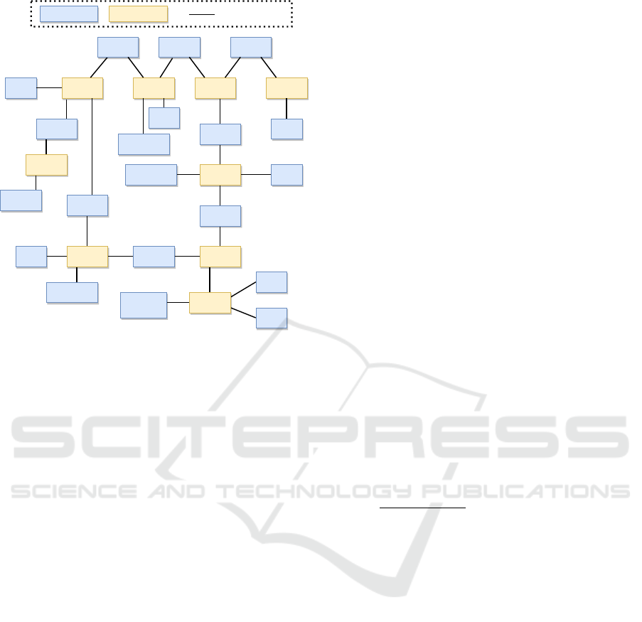
Bus 7 Bus 3

Bus 5

Bus 2

Bus 6

Bus 1

Bus 4

Bus 8 Bus 9

Wind

Line 7-8 Line 8-9

Line 4-6

Line 3-9

Line 6-9

Line 2-7

Line 5-4

Consumer

Line 5-7

Consumer

Wind

Consumer

Wind

External

Tie

Device Agent Net Agent

Communication

Link

PV = Photovoltaic Generator.

Wind = Windturbine Generator.

Line X-Y = Transmission Line between Bus X to Bus Y.

Figure 1: Test Scenario: Agents deployment.

dow that contains a horizon of H = 12 periods of

hourly time-series (half a day) was moved all across

each month of real data. At each step, the window

moves one hour period and the whole set of experi-

ments is run again. We chose three months (January,

May and September) that cover the most representa-

tive climate conditions of a year for the studied re-

gions. In addition, two pairs of buying-selling energy

prices are tested. Buying price corresponds to the cost

of importing energy to the grid from the external util-

ity, and selling price is the cost when energy is ex-

ported. In order to avoid stochastic solutions, each

single experiment was repeated 10 times. Averages

and standard errors are calculated for all the results.

5.2 Device Modeling

To compute the testing scenario, our framework de-

ploys a multi-agent system composed of 18 agents

(one per device/bus of the microgrid) that run their

own local optimisation and negotiate by exchanging

messages. Following the notation of section 3, the

different kinds of devices are modelled as follows:

• Consumers (non controllable) as ﬁxed loads. It

is a single terminal device with zero cost function

) = 0. Considering H as the time horizon of

the optimisation, these devices must satisfy a ex-

pected consumption proﬁle l = [l

(1),...,l

(H)] ∈

at each period, which sets the constraint:

(t) = l

(t), ∀t ∈ [1, ..,H].

• Photovoltaic and wind plants (controllable) as

generators. Single terminal device that generates

power over a range and imposes the constraint

min

(t) ≤ −p

(t) ≤ P

max

(t), ∀t ∈ [1, ...,H] .

The values [P

min

max

] are deﬁned by forecasts.

The cost function is c

) =

∑

t=1

α(−p

(t))

where α > 0.

• Connection to the external power system as ex-

ternal tie. It counts with one terminal and consid-

ers the cost of importing energy from the source

as imp

= [imp

(1),...,imp

(H)] ∈ R

(buying),

and the cost of exporting to the source as exp

[exp

(1),...,exp

(H)] ∈ R

(selling).

We deﬁne its cost function as c

) =

∑

t=1

−η

(t)p

(t) + γ

(t)|p

(t)|, where η

(t) =

(imp

(t) + exp

(t))/2 and γ

(t) = (imp

(t) −

exp

(t))/2, ∀t ∈ [1, ..,H].

• Lines that connect the elements as DC transmis-

sion lines. These devices have two terminals since

they transport power through a distance, which is

also subject to energy losses. Therefore, it has

zero cost function (c

) = 0), but the power

ﬂows are constrained: considering p

as input

power and p

as output power, the line has a

maximum ﬂow capacity given by:

(t) − p

(t)

≥ C

max

,∀t ∈ [1, .., H]

(3)

where C

max

is a capacity constraint. It also

imposes a line loss constraint: p

+ p

−

`(p

, p

) = 0, where `(p

, p

): R

× R

is a loss function.

Following the convention used by Kraning et

al.(Kraning et al., 2014), p

< 0 when a device d is

giving energy to the grid and p

> 0 when consum-

ing.

5.3 Results Discussion

This section reports on the results of the three approx-

imations used:

• Robust Optimisation -Robust Opt-: decentralised

robust optimisation algorithm presented in this

paper (our approach).

• Standard Optimisation -Stand Opt-: decen-

tralised optimisation algorithm for energy net-

works (Kraning et al., 2014) without considering

uncertainty in parameters.

Towards a Robust, Distributed and Decentralised Smart Energy Management of Microgrids

• Non Optimisation -No Opt-: non-optimised ap-

proach were all generators are by default con-

nected at the maximum generation rate. It repre-

sents how a real microgrid would behave without

any smart control.

The three approaches are tested in the same sce-

narios so that their performance results are side-by-

side comparable.

When running the experimentation, we emulated

how the put in practice of the algorithms would be.

First, the optimisation is run relying in forecasted pa-

rameters (real time observations cannot be known a

priori) to get the optimal conﬁgurations (power sched-

ules) and their corresponding cost values. Then, fore-

casts are replaced by real observations and are used

to test such conﬁgurations. Finally, we compare the

deviations in terms of cost that those conﬁgurations

get from forecasted parameters (what it is expected to

ﬁnd) to the observed ones (what it was faced in the

reality).

The results are shown in two tables: i) Table 2

considers exporting the energy selling as almost free,

whereas ii) Table 1 imposes to both exporting or im-

porting energy from the microgrid an associated cost.

These tables show:

• Its.: average number of iterations used by the al-

gorithm to reach the solution.

• Average Cost (C): statistics calculated over the

energy cost, measured in cost units (u). It can

be seen as the average cost across all the exper-

iments. (True currencies and electrical prices are

omitted for the validation phase).

• SEM Cost: the standard deviation of the sample-

mean’s estimate, known as “standard error of the

mean” (Barde and Barde, 2012).Both Average

Cost and SEM Cost are calculated for the same

scenarios using the theoretical situation (fore-

casted parameters) and then the real parameters

(the ones observed a posteriori).

• Cost Saving (CSv): percentage of cost saved when

running the robust optimisation over the stan-

dard optimisation (percentage over its average

cost). Its formula is deﬁned in eq. 4 where C

i, j

is the average cost of the approach i (standard

or robust optimization) using j parameters (fore-

casts//expected or real/observed ones).

CSv =

1 −

real,robust

−C

f orecast,robust

real,stand

−C

f orecast,stand

∗ 100 (4)

Results in Table 1 are computed in the scenarios

where exporting and importing energy from the mi-

crogrid is penalised with 10u. The three tested months

show a similar tendency. We ﬁrst compare a non-

optimised microgrid with the other two approaches to

prove that, in any case, optimisation is always nec-

essary to reduce costs (between 7000 and 42000 (u)

over the non-optimisations). The expected average

costs for standard optimisations in forecast scenarios

differ, in about 1200 (u), from the average of same

schedules but tested with real parameters. However,

robust optimisations yield much smaller deviations.

Actually, the robust optimiser reduces from 6.68% to

60.83% the average cost error over the standard opti-

miser. SEM in tables is low, which indicates few de-

viations over the average (between ±0.1 and ±1.3).

Moreover the number of iterations of both robust and

standard optimisation approaches are similar, which

makes computational effort similar too.

When analysing Table 2 (exporting energy penalty

very low), results show a similar tendency. Aver-

ages and SEMs are usually lower in non optimisa-

tion experiments, which is logical since in this case

exporting energy is almost not penalised. We also ob-

serve that the robust approach gets positive savings

in the three months, from 4.7 to 20.03% of reduc-

tion over the non robust optimisations. September

presents similar cost values as in Table 1, but May and

January are slightly different. May has a similar cost

saving but over lower average and SEM values; this

is probably because in some periods of this scenario

not all the energy produced was consumed and there-

fore it was exported out of the grid. January is the

month with less improvement. It is also the hardest

scenario to be optimised since the optimisers took re-

markably more iterations to solve it, the average costs

are closer (but still smaller) to the non-optimised case,

and SEMs are much higher as well.

Tables 3 and 4 compare the performance of the

three approaches from a different point of view. They

show the proportional cost reduction when optimised

schedules face the real scenarios or, in other words,

“how much the user would save in the real life”. In

general, and as expected, we observe that optimisa-

tions highly outperformed the standard conﬁgurations

of the microgrid. In the same line, power schedules

computed using the robust optimiser originated sig-

niﬁcantly smaller costs than the non robust optimised

solutions and, therefore, such difference was bigger

when compared to the basic (non optimised) conﬁgu-

rations of the microgrid.

A question that raises observing the results is why

the percentage of saving cost varies up to 15% de-

pending of the months. This is due to the variation of

the weather conditions and, in consequence, the max-

imum capacity of production. Furthermore, each sce-

nario presents different ﬂexibilities, allowing differ-

ICAART 2022 - 14th International Conference on Agents and Artiﬁcial Intelligence

Table 1: Experimental results for energy costs: selling = 10(u/kW); buying = 10(u/kW).

Approach Its.

Average Cost (u) SEM Cost (u) CSv

(%)Forecasts Real Forecasts Real

January

No Opt – – 14337.6350 – 54.1596

Stand Opt 302 212.3893 317.4002 0.0276 0.3795

Robust Opt 302 278.6910 319.8174 0.1968 0.2539 60.83

May

No Opt – – 8935.7970 – 27.2481

Stand Opt 484 0.0000 1344.7288 0.0000 0.0408

Robust Opt 421 0.0002 1079.0624 0.0000 0.1037 19.75

September

No Opt – – 12172.7330 – 317.7966

Stand Opt 583 660.3829 2044.1316 0.5466 1.3871

Robust Opt 561 655.6976 1947.0089 0.5607 0.0193 6.68

Table 2: Experimental results for energy costs: selling = 1(u/kW); buying = 10(u/kW).

Approach Its.

Average Cost (u) SEM Cost (u) CSv

(%)Forecasts Real Forecasts Real

January

No Opt – – 2581.5314 – 182.1753

Stand Opt 1694 285.3534 2232.0703 29.3623 112.9993

Robust Opt 1607 273.1762 2128.1336 28.6996 111.1019 4.71

May

No Opt – – 6052.6184 – 374.7932

Stand Opt 421 0.0051 133.3903 0.0001 0.1081

Robust Opt 428 0.0080 106.6703 0.0002 0.0835 20.03

September

No Opt – – 10300.3550 – 465.0780

Stand Opt 1445 681.2515 2043.7722 0.9455 1.5547

Robust Opt 2158 682.8970 1955.0863 0.9505 0.1233 6.62

Table 3: Cost Saving (%) of Table 1.

10/10

No Opt Stand Opt

Jan. May Sept. Jan. May Sept.

Stand Opt 97.78 84.95 83.20 – – –

Robust Opt 97.76 87.92 84.00 -0.76 19.75 4.75

Table 4: Cost Saving (%) of Table 2.

1/10

No Opt Stand Opt

Jan. May Sept. Jan. May Sept.

Stand Opt 13.53 97.79 80.15 – – –

Robust Opt 17.56 98.23 81.01 4.65 20.03 4.33

ent degrees of optimisations. Note that the proposed

approach is more effective in more ﬂexible scenarios

where the algorithm has more freedom to control. For

instance, in a scenario in which all devices that rely on

forecasts can be fully controlled, the robust optimisa-

tion would outperform the standard one. However,

low level of ﬂexibility will tend to approach robust

optimisations costs to standard optimisation ones. In

conclusion: the more ﬂexible the scenario it is, the

greater cost can be saved.

Summarising, Tables 1 to 4 showed how, for all

experiments, the robust optimisation provided micro-

grid conﬁgurations (power schedules) with the lowest

cost values. The same way, such approach performed

better when facing more ﬂexible scenarios.

6 CONCLUSIONS AND FUTURE

LINES

In the last decades the interests and efforts for bring-

ing intelligence to conventional power grids are in-

creasing more and more. The emerge of smart grids

with distributed electrical resources keeps calling for

automatic, and distributed, control which looks for the

best decisions to make. Such search usually poses an

optimisation problem where the looking for good so-

lutions is gaining track in the research ﬁeld. Many

algorithms have been proposed in the literature but

only few of them can operate in a distributed manner.

Moreover, when the solutions are schedules that shall

be used in the near future, forecasts are usually con-

sidered in the optimisation process. Unfortunately,

forecasts are never 100% accurate and, as a conse-

quence, optimisations are not usually reliable.

We propose a decentralised optimisation algo-

rithm that, implemented in a distributed manner by

Towards a Robust, Distributed and Decentralised Smart Energy Management of Microgrids

a multi-agent system, considers the uncertainty of the

parameters in the optimisation process. Our approach

deals with such uncertainty through a robust mecha-

nism which is added to the optimiser. Our solution

was tested and compared with the base line showing

the efﬁciency of this technique since the costs of the

optimized schedules computed for all tested scenarios

were signiﬁcantly reduced.

Our approach can be extended in many directions

in the future: i.e., it would be interesting to explore the

optimisation from a multiobjective point of view by

considering several goals. Another interesting study

would be the collective uncertainty; i.e., to study how

forecasts of devices situated nearby by could present

the same deviations tendency. Finally, a software

analysis on how to implement and deploy the ap-

proach in a real microgrid is also a step to follow.

ACKNOWLEDGEMENTS

This work was supported by the European Commu-

nity’s Seventh Framework Programme under Grant

Agreement no. 619682 (Project MAS2TERING) and

by ITEA 2 call 8 (Project 13023 FUSE-IT).

REFERENCES

Al-Hinai, A. and Alhelou, H. H. (2021). A multi-agent

system for distribution network restoration in future

smart grids. Energy Reports.

Amin, S. and Wollenberg, B. (2005). Toward a smart grid:

Power delivery for the 21st century. IEEE Power En-

ergy Mag, 3:34 – 41.

Auger, A., Schoenauer, M., and Vanhaecke, N. (2004).

Ls-cma-es: A second-order algorithm for covariance

matrix adaptation. In Parallel Problem Solving from

Nature-PPSN VIII, pages 182–191. Springer.

Barde, M. P. and Barde, P. J. (2012). What to use to ex-

press the variability of data: Standard deviation or

standard error of mean? Perspectives in clinical re-

search, 3(3):113.

Boyd, S., Parikh, N., Chu, E., Peleato, B., and Eck-

stein, J. (2011). Distributed Optimization and Statis-

tical Learning via the Alternating Direction Method

of Multipliers. Foundations and Trends in Machine

Learning, 3(1):1–122.

Chakraborty, S. and Okabe, T. (2016). Robust energy

storage scheduling for imbalance reduction of strate-

gically formed energy balancing groups. Energy,

114:405–417.

Chen, G.-c. and Yu, J.-s. (2005). Particle swarm optimiza-

tion algorithm. INFORMATION AND CONTROL-

SHENYANG-, 34(3):318.

Colak, I., Sagiroglu, S., Fulli, G., Yesilbudak, M., and Cov-

rig, C.-F. (2016). A survey on the critical issues in

smart grid technologies. Renewable and Sustainable

Energy Reviews, 54:396 – 405.

Dantzig, G. B. and Wolfe, P. (1960). Decomposition

principle for linear programs. Operations research,

8(1):101–111.

de Cerio Mendaza, I. D., Szczesny, I. G., Pillai, J. R., and

Bak-Jensen, B. (2016). Demand response control in

low voltage grids for technical and commercial aggre-

gation services. IEEE Transactions on Smart Grid,

7(6):2771–2780.

Deb, K., Pratap, A., Agarwal, S., and Meyarivan, T. (2002).

A fast and elitist multiobjective genetic algorithm:

NSGA-II. IEEE Transactions on Evolutionary Com-

putation, 6(2):182–197.

Deconinck, G., Vanthournout, K., Beitollahi, H., Qui, Z.,

Duan, R., Nauwelaers, B., Van Lil, E., Driesen, J., and

Belmans, R. (2008). A robust semantic overlay net-

work for microgrid control applications. In Architect-

ing Dependable Systems V, pages 101–123. Springer.

Dehghanpour, K., Nehrir, H., Sheppard, J., and Kelly, N.

(2017). Agent-based modeling of retail electrical en-

ergy markets with demand response. IEEE Transac-

tions on Smart Grid.

Diekerhof, M., Peterssen, F., and Monti, A. (2017). Hi-

erarchical distributed robust optimization for demand

response services. IEEE Transactions on Smart Grid.

Diekerhof, M., Schwarz, S., and Monti, A. (2016).

Distributed optimization for electro-thermal heating

units. In PES Innovative Smart Grid Technologies

Conference Europe (ISGT-Europe), 2016 IEEE, pages

1–6. IEEE.

Diekerhof, M., Vorkampf, S., and Monti, A. (2014).

Distributed optimization algorithm for heat pump

scheduling. In Innovative Smart Grid Technologies

Conference Europe (ISGT-Europe), 2014 IEEE PES,

pages 1–6. IEEE.

Farhangi, H. (2010). The path of the smart grid. IEEE

Power Energy Mag, 8:18 – 28.

Gamarra, C. and Guerrero, J. M. (2015). Computational op-

timization techniques applied to microgrids planning:

a review. Renewable and Sustainable Energy Reviews,

48:413–424.

Garc

ıa, S., Quintana, D., Galv

an, I. M., and Isasi, P.

(2012). Time-stamped resampling for robust evolu-

tionary portfolio optimization. Expert Systems with

Applications, 39(12):10722–10730.

Garcia-Rodriguez, S., Sleiman, H. A., and Nguyen, V.-Q.-

A. (2016). A multi-agent system architecture for mi-

crogrid management. In Trends in Practical Appli-

cations of Scalable Multi-Agent Systems, the PAAMS

Collection, pages 55–67. Springer International Pub-

lishing.

Gomez-Sanz, J. J., Garcia-Rodriguez, S., Cuartero-Soler,

N., and Hernandez-Callejo, L. (2014). Reviewing mi-

crogrids from a multi-agent systems perspective. En-

ergies, 7(5):3355–3382.

Haring, T. W., Mathieu, J. L., and Andersson, G. (2016).

Comparing centralized and decentralized contract de-

ICAART 2022 - 14th International Conference on Agents and Artiﬁcial Intelligence

sign enabling direct load control for reserves. IEEE

Transactions on Power Systems, 31(3):2044–2054.

Kraning, M., Chu, E., Lavaei, J., and Boyd, S. (2014). Dy-

namic network energy management via proximal mes-

sage passing. Foundations and Trends in Optimiza-

tion, 1(2):73–126.

Liang, H. and Zhuang, W. (2014). Stochastic modeling

and optimization in a microgrid: A survey. Energies,

7(4):2027–2050.

Mahat, P., Escribano Jim

enez, J., Moldes, E. R., Haug,

S. I., Szczesny, I. G., Pollestad, K. E., and Totu, L. C.

(2013). A micro-grid battery storage management. In

2013 IEEE PES General Meeting.

McArthur, S. D., Davidson, E. M., Catterson, V. M.,

Dimeas, A. L., Hatziargyriou, N. D., Ponci, F., and

Funabashi, T. (2007a). Multi-agent systems for

power engineering applications-part i: Concepts, ap-

proaches, and technical challenges. IEEE Transac-

tions on Power systems, 22(4):1743–1752.

McArthur, S. D., Davidson, E. M., Catterson, V. M.,

Dimeas, A. L., Hatziargyriou, N. D., Ponci, F., and

Funabashi, T. (2007b). Multi-agent systems for power

engineering applications-part ii: Technologies, stan-

dards, and tools for building multi-agent systems.

IEEE Transactions on Power Systems, 22(4):1753–

1759.

McNamara, P. and McLoone, S. (2015). Hierarchical de-

mand response for peak minimization using dantzig–

wolfe decomposition. IEEE Transactions on Smart

Grid, 6(6):2807–2815.

Mesaric, P., Dukec, D., and Krajcar, S. (2017). Exploring

the potential of energy consumers in smart grid using

focus group methodology. Sustainability, 9(8):1463.

Meyn, S. P., Barooah, P., Bu

c, A., Chen, Y., and Ehren,

J. (2015). Ancillary service to the grid using intel-

ligent deferrable loads. IEEE Transactions on Auto-

matic Control, 60(11):2847–2862.

Mihaylov, M., R

adulescu, R., Razo-Zapata, I., Jurado, S.,

Arco, L., Avellana, N., and Now

e, A. (2019). Com-

paring stakeholder incentives across state-of-the-art

renewable support mechanisms. Renewable energy,

131:689–699.

Moghaddam, A. A., Seiﬁ, A., Niknam, T., and Pahlavani,

M. R. A. (2011). Multi-objective operation manage-

ment of a renewable {MG} (micro-grid) with back-up

micro-turbine/fuel cell/battery hybrid power source.

Energy, 36(11):6490 – 6507.

Mohamed, F. A. and Koivo, H. N. (2007). System mod-

elling and online optimal management of microgrid

using multiobjective optimization. In Clean Electri-

cal Power, 2007. ICCEP’07. International Conference

on, pages 148–153. IEEE.

Moreno, R., Street, A., Arroyo, J. M., and Mancarella,

P. (2017). Planning low-carbon electricity systems

under uncertainty considering operational ﬂexibility

and smart grid technologies. Phil. Trans. R. Soc. A,

375(2100):20160305.

National Renewable Energy Laboratory (2006a). So-

lar integration data sets. https://www.nrel.gov/grid/

solar-integration-data.html.

National Renewable Energy Laboratory (2006b). Wind

integration data sets. https://www.nrel.gov/grid/

wind-integration-data.html.

Paul M. Anderson, A. A. F. (2003). Power System Control

and Stability, 2nd. IEEE Press, New York.

Ramaswamy, P. and Deconinck, G. (2012). Smart grid

reconﬁguration using simple genetic algorithm and

nsga-ii. In Innovative Smart Grid Technologies (ISGT

Europe), 2012 3rd IEEE PES International Confer-

ence and Exhibition on, pages 1–8.

Rivera, J., Goebel, C., and Jacobsen, H.-A. (2017). Dis-

tributed convex optimization for electric vehicle ag-

gregators. IEEE Transactions on Smart Grid.

Saad, W., Han, Z., Poor, H. V., and Basar, T. (2012). Game-

theoretic methods for the smart grid: An overview

of microgrid systems, demand-side management, and

smart grid communications. IEEE Signal Processing

Magazine, 29(5):86–105.

Sanseverino, E. R., Di Silvestre, M. L., Ippolito, M. G.,

De Paola, A., and Re, G. L. (2011). An execution,

monitoring and replanning approach for optimal en-

ergy management in microgrids. Energy, 36(5):3429–

3436.

Storn, R. and Price, K. (1997). Differential evolution–a

simple and efﬁcient heuristic for global optimization

over continuous spaces. Journal of global optimiza-

tion, 11(4):341–359.

Tajalli, S. Z., Kavousi-Fard, A., Mardaneh, M., Khosravi,

A., and Razavi-Far, R. (2021). Uncertainty-aware

management of smart grids using cloud-based lstm-

prediction interval. IEEE Transactions on Cybernet-

ics.

Tuballa, M. L. and Abundo, M. L. (2016). A review of the

development of smart grid technologies. Renewable

and Sustainable Energy Reviews, 59:710 – 725.

Veldman, E., Gibescu, M., Slootweg, H. J., and Kling, W. L.

(2013). Scenario-based modelling of future residen-

tial electricity demands and assessing their impact on

distribution grids. Energy Policy, 56:233–247.

Zhang, J., Zhan, Z.-h., Lin, Y., Chen, N., Gong, Y.-j.,

Zhong, J.-h., Chung, H. S., Li, Y., and Shi, Y.-h.

(2011). Evolutionary computation meets machine

learning: A survey. IEEE Computational Intelligence

Magazine, 6(4):68–75.

Zhang, Y. and Giannakis, G. B. (2016). Distributed stochas-

tic market clearing with high-penetration wind power.

IEEE Transactions on Power Systems, 31(2):895–906.

Zhang, Y., Shen, S., and Mathieu, J. L. (2017). Distribu-

tionally robust chance-constrained optimal power ﬂow

with uncertain renewables and uncertain reserves pro-

vided by loads. IEEE Transactions on Power Systems,

32(2):1378–1388.

Zitzler, E., Laumanns, M., and Thiele, L. (2001). SPEA2:

Improving the strength pareto evolutionary algorithm.

Technical Report 103, Computer Engineering and

Networks Laboratory (TIK), Swiss Federal Institute

of Technology (ETH), Zurich, Switzerland.

Towards a Robust, Distributed and Decentralised Smart Energy Management of Microgrids