Time Series Augmentation based on Beta-VAE to Improve Classiﬁcation

Performance

Domen Kavran, Borut

Zalik and Niko Luka

Faculty of Electrical Engineering and Computer Science, University of Maribor, Koro

ska ulica 46, Maribor, Slovenia

Keywords:

Time Series, Augmentation, Classiﬁcation, Variational Autoencoder, Beta-VAE.

Abstract:

Classiﬁcation models that provide good generalization are trained with sufﬁciently large datasets, but these

are often not available due to restrictions and limited resources. A novel augmentation method is presented

for generating synthetic time series with Beta-VAE variational autoencoder, which has ResNet-18 inspired

architecture. The proposed augmentation method was tested on benchmark univariate time series datasets. For

each dataset, multiple variational autoencoders were used to generate different amounts of synthetic time series

samples. These were then used, along with the original train set samples, to train MiniRocket classiﬁcation

models. By using the proposed augmentation method, a maximum increase of 1,22% in classiﬁcation accuracy

was achieved on the tested datasets in comparison to baseline results, which were obtained by training only

with original train sets. An increase of up to 0,81% in accuracy of simple machine learning classiﬁers was

observed by benchmarking the proposed augmentation method with the 1-nearest neighbor algorithm.

1 INTRODUCTION

Technologically advanced industries generate

structured and unstructured big data with various

device-mounted sensors and software tools. Year by

year the rise in quantity of big data is correlated with

the expansion of Internet of Things (IoT) devices.

Their integration ranges from home appliances and

medical equipment to construction machines and

Unmanned Aerial Vehicles (UAVs). One of the most

common data types are time series. Large quantities

of time series are produced in the medical, automotive

and ﬁnancial industries (Lines et al., 2017). Time

series contain measurements of observed quantities

over time, most commonly being physical quantities

(e.g. electric current, and temperature) and web

activity (e.g. media streaming). Analysis of time

series is challenging, because the acquired time series

can be high-dimensional, noisy, and may contain data

gaps (Gian Antonio et al., 2018).

Time series classiﬁcation is an important part of

many advanced software applications, ranging from

identiﬁcation of various anomalies and safety hazards

to recognition of medical conditions and diseases

(Lines et al., 2017). Large time series datasets are

needed to train robust state-of-the-art classiﬁcation

models. Datasets are most commonly prepared

by domain experts, who hand label collected data.

That approach is time consuming, and expensive for

larger amounts of samples. Often many samples are

not available for experts to label, which harms the

generalization property of the trained models. To

solve the described problems, hand labeling can still

be performed on smaller, representative sets of time

series, although these are then used for augmentation

methods to create additional samples to be used

in the training process. Time series augmentations

are not as trivial as image augmentation techniques

(e.g. cropping, rotating, scaling), because changes

in time series can deteriorate underlying properties

of the original data (Oh et al., 2020). An alternative

approach for augmentations is generation of synthetic

data with generative models.

The proposed paper presents a novel

augmentation method for generating synthetic

time series with a residual neural network (ResNet)

based variational autoencoder, which applies

stronger constraint on the latent bottleneck, thus

making encodings disentangled. By manipulating

disentangled latent factors, individual time series

characteristics are controlled to generate new time

series samples. These are then, along with the

original train data, used for training classiﬁcation

models. In the presented paper, the MiniRocket

classiﬁcation algorithm was used, due to its low

computational complexity (Dempster et al., 2020).

Kavran, D., Žalik, B. and Luka

c, N.

Time Series Augmentation based on Beta-VAE to Improve Classiﬁcation Performance.

DOI: 10.5220/0010749200003116

In Proceedings of the 14th International Conference on Agents and Artiﬁcial Intelligence (ICAART 2022) - Volume 2, pages 15-23

ISBN: 978-989-758-547-0; ISSN: 2184-433X

This paper consists of ﬁve sections. The

next section presents related work about

state-of-the-art time series classiﬁcation algorithms

and augmentation methods. The third section

presents the proposed augmentation method for

generating synthetic time series samples. In the same

section, we also present the MiniRocket classiﬁcation

algorithm. The effects of sythetic time series on

classiﬁcation performance are presented in the fourth

section. The conclusions are given in the last section.

2 RELATED WORK

In this section, we ﬁrst present current state-of-the-art

time series classiﬁcation algorithms. Advanced

augmentation methods for time series data are

presented in subsection 2.2.

2.1 Time Series Classiﬁcation

Many state-of-the-art classiﬁcation algorithms have

been developed in recent years. Hierarchical Vote

Collective of Transformation-based Ensembles

(HIVE-COTE) is an ensemble of time series

classiﬁers, trained in multiple domains, including

shapelets and bag-of-words dictionaries (Lines

et al., 2017). HIVE-COTE achieved the highest

classiﬁcation accuracies on benchmark datasets

compared to other state-of-the-art classiﬁers,

although it has very high computational complexity,

which makes it impractical to use in real-world

applications. A deep learning ensemble of ﬁve deep

Convolutional Neural Networks (CNNs), named

InceptionTime, has proven to achieve state-of-the-art

classiﬁcation accuracies, while having much

lower training time complexity than HIVE-COTE

(Ismail Fawaz et al., 2020). Rocket, and its improved

version MiniRocket, are algorithms which achieve

state-of-the-art time series classiﬁcation accuracies.

Both have very low computational complexity, but

MiniRocket is capable of being up to 75 times

faster than Rocket, while still achieving essentially

the same accuracy (Dempster et al., 2020). The

recently developed HIVE-COTE 2.0 introduces

improvements to the original HIVE-COTE with

additional classiﬁers, including Rocket, to achieve

higher classiﬁcation scores (Middlehurst et al., 2021).

2.2 Time Series Augmentation Methods

Multiple advanced time series augmentations, called

AddNoise, Permutation, Scaling and Warping, have

been proposed, in order to improve time series

classiﬁcation with the Fully Convolutional Neural

Network (FCN) and residual neural network (ResNet)

(Liu et al., 2020). Of all these augmentations,

at least one always improved the accuracy of the

trained model, but certain combinations of combined

augmentations have also made the classiﬁcation

accuracy worse. A recently developed time

series augmentation based on interpolation has the

advantage of low computational complexity, and

has proven to beneﬁt the models to achieve higher

classiﬁcation accuracies on benchmark datasets (Oh

et al., 2020).

Augmentations can also be performed with

generative models, which are classiﬁed into two

categories - statistical models and neural network-

based models. Statistical models are often used

to enlarge training datasets to improve time series

forecasting. Time series generation models, based on

the Local and Global Trend (LGT) forecasting model,

have been shown to improve forecasting results.

GeneRAting TImeSeries (GRATIS) is a method

which uses mixture autoregressive models to simulate

time series. Neural network-based generative models

are divided into encoder-decoder networks and

generative adversarial networks (GANs). Encoder-

decoder networks for time series generation are

represented by long short-term memory (LSTM)

based autoencoders and variational autoencoders.

The underlying GAN networks are separated

into four architectures, which are either based

on fully-connected networks, residual networks,

temporal one-dimensional convolutional networks,

or two-dimensional convolutional networks, that

generate frequency spectra. Speciﬁed architectures

can be combined into various hybrid GAN networks

(Iwana and Uchida, 2021).

3 TIME SERIES GENERATION

AND CLASSIFICATION

The time series generation is performed with a

variational autoencoder (VAE), called Beta-VAE,

which discovers interpretable latent representations

from raw time series data (Higgins et al., 2017). By

sampling randomly from a Gaussian distribution, a

new latent representation is created and decoded by

the variational autoencoder. The decoded output is a

generated time series, similar to the time series which

were used for training the variational autoencoder.

Original training time series samples are used for

training Beta-VAE variational autoencoders. One

variational autoencoder has to be trained individually

for each classiﬁcation class that needs additional

ICAART 2022 - 14th International Conference on Agents and Artiﬁcial Intelligence

synthetic time series samples. Samples in the

validation set are used to validate variational

autoencoders and a MiniRocket classiﬁer during their

training process. Trained Beta-VAEs are used to

generate synthetic time series samples, which are then

stored in a synthetic set. Both train and synthetic sets

are used for training the MiniRocket classiﬁer. The

learned classiﬁcation model is tested with a test set.

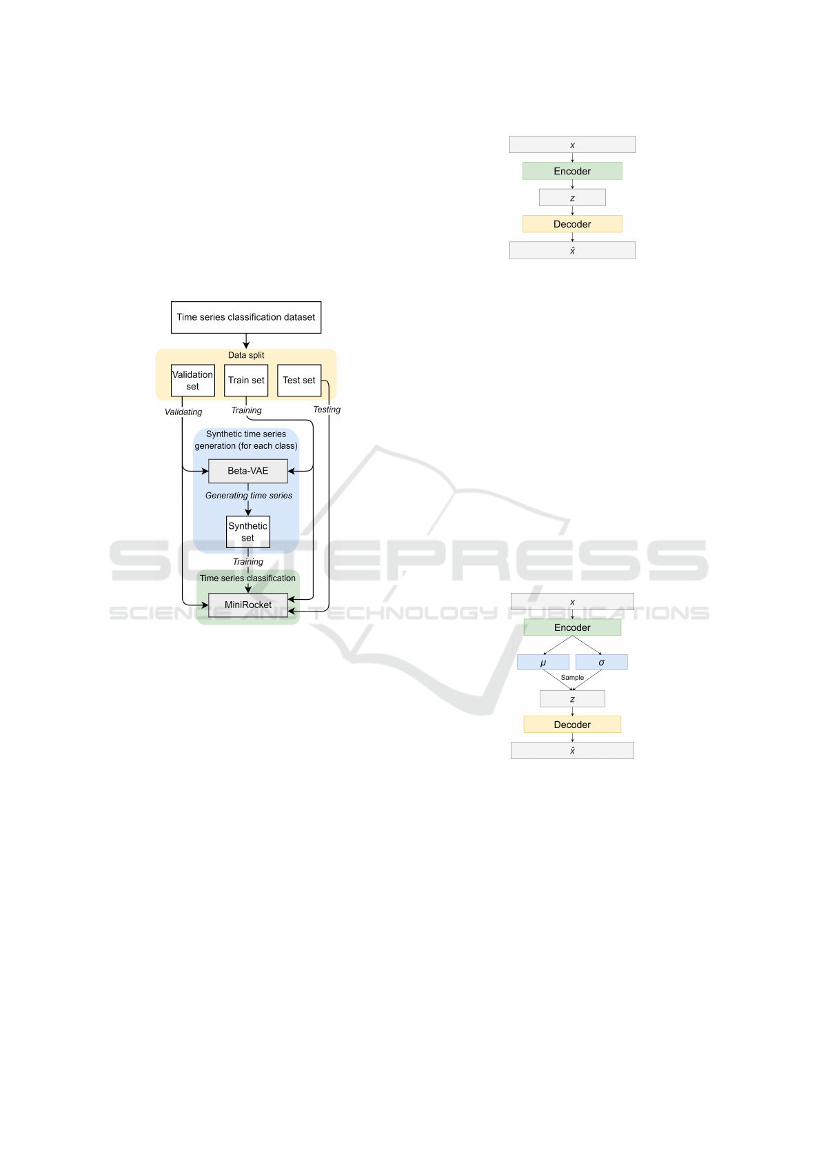
Figure 1 shows the described workﬂow, which starts

by splitting data into multiple sets.

Figure 1: Time series generation and classiﬁcation

workﬂow for individual time series classiﬁcation dataset.

The autoencoders and the proposed Beta-VAE

architecture are described in the next subsection,

while the classiﬁcation algorithm MiniRocket is

presented in subsection 3.2.

3.1 Time Series Generation

3.1.1 Autoencoder

An autoencoder is a dimensionality reduction

model, that consists of two neural networks.

The encoding neural network, called encoder,

performs dimensionality reduction of the input data

x. Compressed data, also referred to as latent

representation z of size z

dim

, is reconstructed using

the decoding neural network, called decoder. The

autoencoder architecture is shown in Figure 2.

During the training of an autoencoder, a

reconstruction loss (e.g. mean squared error,

mean average error, and categorical cross-entropy)

Figure 2: Autoencoder architecture.

is used to minimize the difference between input

x and the reconstruction ˆx (Bank et al., 2020).

Latent representations capture the most signiﬁcant

features of the input data, which makes autoencoders

useful for data compression and anomaly detection

applications (Bank et al., 2020).

3.1.2 Variational Autoencoder (VAE)

A variational autoencoder is a probabilistic generative

model. It has a similar architecture to an autoencoder

with additional hidden layers - mean layer µ and

Standard Deviation layer σ (Kingma and Welling,

2014). Input x conditions the latent representation

z, which is retrieved by sampling the Gaussian

distribution N , parameterized by µ and σ. The

variational autoencoder architecture is shown in

Figure 3.

Figure 3: Variational autoencoder architecture.

Latent representation sampling is written by

(1) (Sadati et al., 2019). A reparameterization

trick is performed, because sampling of the latent

representation z is stochastic. It introduces a

parameterless random variable ε, sampled from

standard Gaussian distribution. The procedure of

obtaining latent distribution z is altered - instead of

sampling the distribution, z is obtained by (2), with

 symbolizing element-wise product (Kingma and

Welling, 2014).

z ∼ N (µ, σ

) (1)

Time Series Augmentation based on Beta-VAE to Improve Classiﬁcation Performance

z = µ + σ  ε, ε ∼ N (0, 1) (2)

The described process keeps µ and σ learnable during

backpropagation, and maintains the stochasticity of

the latent bottleneck z.

Loss L for the variational autoencoder consists of

two parts - reconstruction term L

, which measures

the error between x and ˆx, and the Kullback-Leibler

divergence term L

, which measures how a

probability distribution is different from a reference

distribution. By introducing the divergence term into

the loss function, the variational autoencoder learns

a standard normal latent space distribution. The

described loss is written by (3)

L = L

(x, ˆx) + L

(p(z|x), p(z)) (3)

where p(z|x) is the conditional distribution of the

encoder, and p(z) is N (0, 1) (Liu et al., 2019).

Generation of a new sample starts by sampling the

standard Gaussian distribution. The sampled latent

representation z is then passed into the decoder to

generate a new sample, similar to training data.

3.1.3 Beta-VAE

Latent representation z is disentangled if each unit is

sensitive to a single generative factor and invariant

to other factors. The described latent representations

are more interpretable. For example, individual

latent units in a variational autoencoder, trained on a

medical time series (e.g. ECG and EEG), can capture

abrupt changes, seasonality and short-lasting trends.

By making latent representations disentangled, latent

encodings become more efﬁcient, which makes

generation of new data easier to control (Higgins

et al., 2017).

Beta-VAE is a variational autoencoder intended

for discovering disentangled latent factors. It has

the same basic architecture as a regular variational

autoencoder, with the only difference being the

introduction of hyperparameter β to the loss function,

written by (4) (Higgins et al., 2017).

L = L

(x, ˆx) + βL

(p(z|x), p(z)) (4)

The weight of the Kullback-Leibler divergence term

is adjusted with β. By increasing β above

a value of 1, a stronger constraint is applied on

latent bottleneck z, thus limiting its representation

capacity, making latent encodings more efﬁcient,

which results in better disentanglement. Models

trained with higher β values may produce poor

quality reconstructions - excessive blurring is often

present (Higgins et al., 2017). Disentangled latent

representations have become one of the main research

areas of unsupervised deep learning.

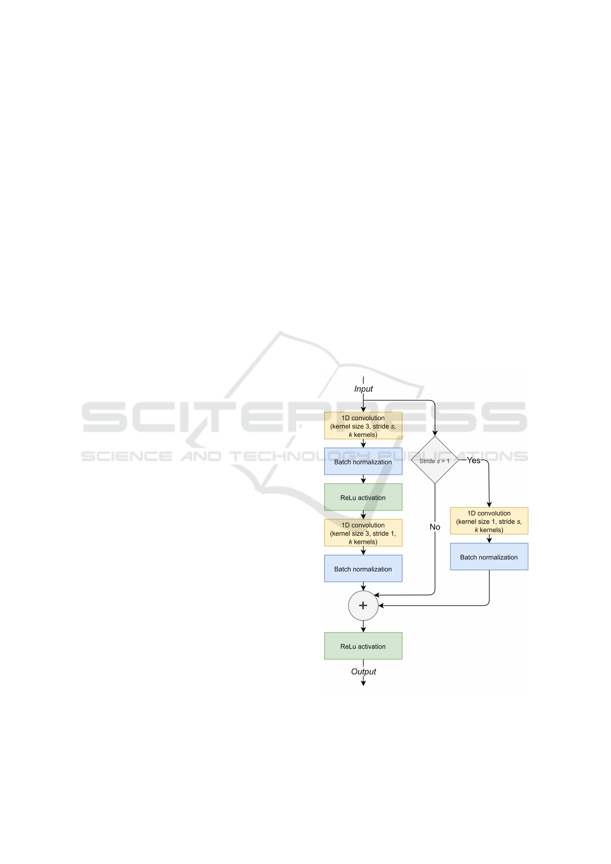
3.1.4 Proposed Beta-VAE Architecture

The encoder and decoder in the proposed Beta-VAE

architecture are 18-layer residual networks (ResNets),

adapted for time series (Wang et al., 2017). Residual

blocks are joined sequentially in a residual layer. The

size of the input x and output ˆx equals the ﬁxed

length T of the time series. The minimal input time

series length is 8, because three residual layers in

the encoder perform convolutions with stride s = 2,

which results in the output being eight times smaller

than T . The decoder’s residual layers reverse the

downsampling effects by performing three upscale

interpolations by a factor sf = 2. If the time series

length is not divisible by 8, it should be zero padded.

ResNet-18 encoder and decoder blocks are shown

in Figures 4 and 5, where Input

channels

represents

the number of channels in the input Input to the

block. The proposed Beta-VAE architecture is shown

in Table 1.

Figure 4: ResNet-18 encoder block.

ICAART 2022 - 14th International Conference on Agents and Artiﬁcial Intelligence

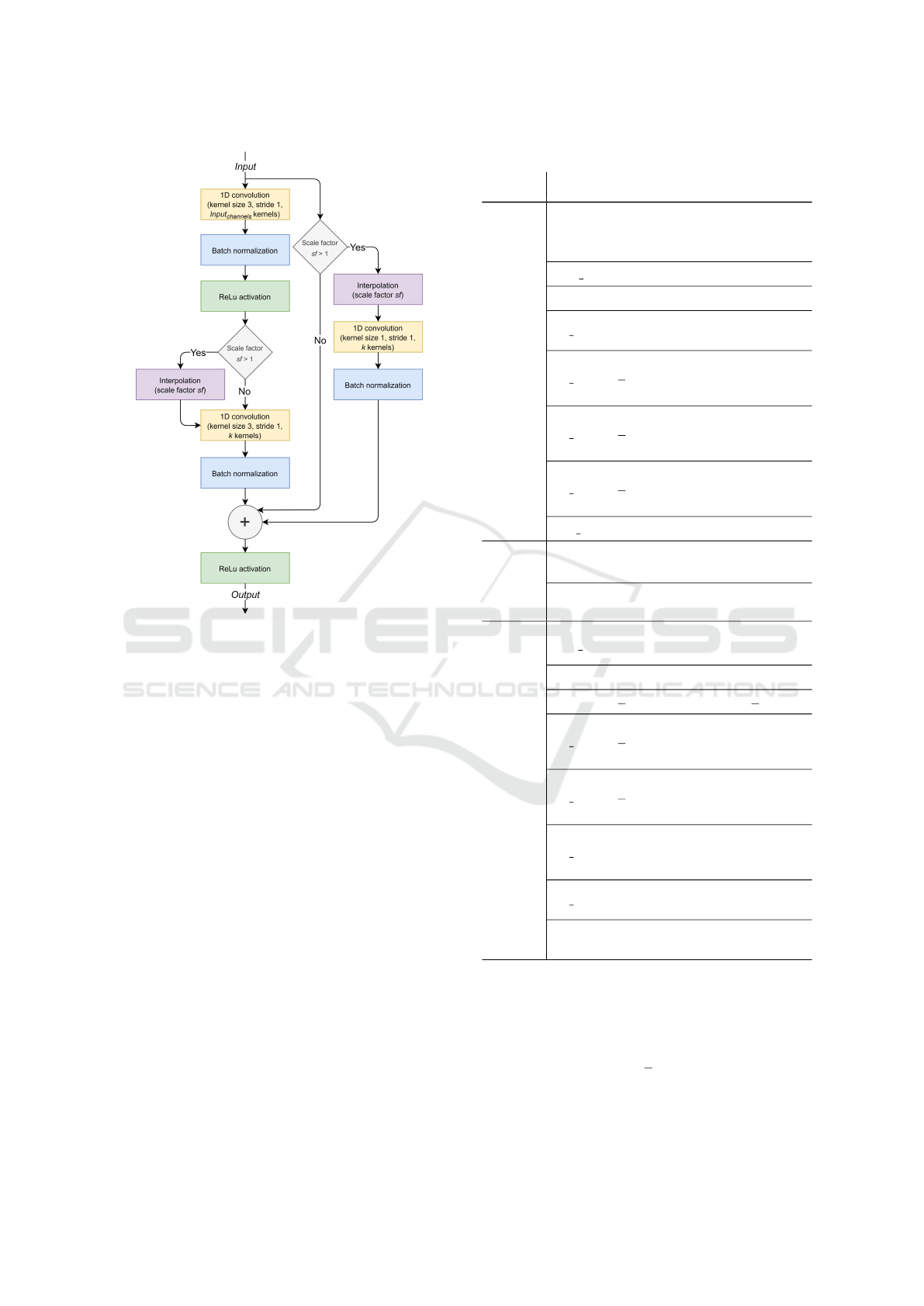
Figure 5: ResNet-18 decoder block.

3.2 Time Series Classiﬁcation

Algorithm

MiniRocket (MINImally RandOm Convolutional

KErnel Transform), is a state-of-the-art time series

classiﬁcation method (Dempster et al., 2020). The

advantages of the method are execution speed and

low computational expense, while still achieving high

classiﬁcation accuracy scores on benchmark datasets.

The core of the MiniRocket method is feature

extraction. It starts by convolving each time series

with a ﬁxed set of kernels of length 9. Each kernel

has weights containing values either -1 or 2. Kernels

are restricted by containing exactly 3 values of 2. The

sum of weights for each kernel is 0. 84 unique kernels

are created based on these restrictions. The only

random component of the method is the kernel bias

hyperparameter - each kernel’s bias is set by drawing

from the quantiles of the convolution output for a

randomly selected training sample. The maximum

number of dilations per kernel is 32, because larger

dilation values do not improve classiﬁcation accuracy,

and make feature extraction less efﬁcient. Half of

the kernel/dilation combinations use zero padding,

and the other half do not. The pooling method

Table 1: Proposed Beta-VAE Architecture.

Stage

Layer

name

Output

size

Description

ResNet-18

encoder

(sequential

layers)

conv1 T ×64

Convolution with kernel

size 3, stride 1, 64

kernels

batch norm T ×64 Batch normalization

relu T ×64 ReLu activation

res layer1 T ×64

Residual layer

(s=1, k=64)×2 blocks

res layer2

×128

Residual layer

(s=2, k=128)×1 block

(s=1, k=128)×1 block

res layer3

×256

Residual layer

(s=2, k=256)×1 block

(s=1, k=256)×1 block

res layer4

×512

Residual layer

(s=2, k=512)×1 block

(s=1, k=512)×1 block

avg pool 512 Average pool

Bottleneck

µ z

dim

512×z

dim

fully

connected layer

σ z

dim

512×z

dim

fully

connected layer

ResNet-18

decoder

(sequential

layers)

fully conn 8192

dim

×8192 fully

connected layer

reshape 16×512 Reshape to 16×512

interp

×512 Interpolate to

×512

res layer5

×256

Residual layer

(s f =2, k=256)×1 block

(s f =1, k=256)×1 block

res layer6

×128

Residual layer

(s f =2, k=128)×1 block

(s f =1, k=128)×1 block

res layer7 T ×64

Residual layer

(s f =2, k=64)×1 block

(s f =1, k=64)×1 block

res layer8 T ×64

Residual layer

(s f =1, k=64)×2 blocks

conv2 T

Convolution with kernel

size 3, stride 1, 1 kernel

’proportion of positive values’ (PPV) is performed

after convolution. It is deﬁned by (5) (Dempster et al.,

2020). Feature extraction results in 10,000 features.

PPV (X ∗W − b) =

∑

[X ∗W − b > 0] (5)

The efﬁciency and execution speed of feature

extraction is possible by taking advantage of a small,

Time Series Augmentation based on Beta-VAE to Improve Classiﬁcation Performance

ﬁxed set of two-valued kernels and smart calculation

of PPV. Optimizations are performed by computing

PPV for W and −W at the same time, not using

multiplications in the convolution operations, reusing

the convolution output to compute multiple features

and for each dilation, computing all kernels (almost)

’at once’. The extracted features are used to train a

linear classiﬁer - either a ridge regression classiﬁer

or logistic regression, if the train set contains more

than 10,000 time series samples. In its general form,

MiniRocket feature extraction applies k kernels on

n number of time series samples of l length, which

results in linear computational complexity O(k · n · l)

(Dempster et al., 2020).

4 RESULTS

Time series classiﬁcation was performed on a subset

of univariate UAE & UCR datasets (Bagnall et al.,

2021). The used datasets are presented in Table 2.

Each dataset contains time series of ﬁxed lengths and

has a predeﬁned train and test set. For each dataset,

synthetic time series samples for each class were

generated by Beta-VAEs with z

dim

=64 latent factors.

This number of latent factors was chosen because it

is less than the shortest time series length of 84 in the

featured datasets. Each variational autoencoder was

trained for 250 epochs with β = 2. A large number of

epochs was selected, to ensure each autoencoder was

trained until convergence. Increasing the parameter

β > 2 had a negligible effect on training losses and

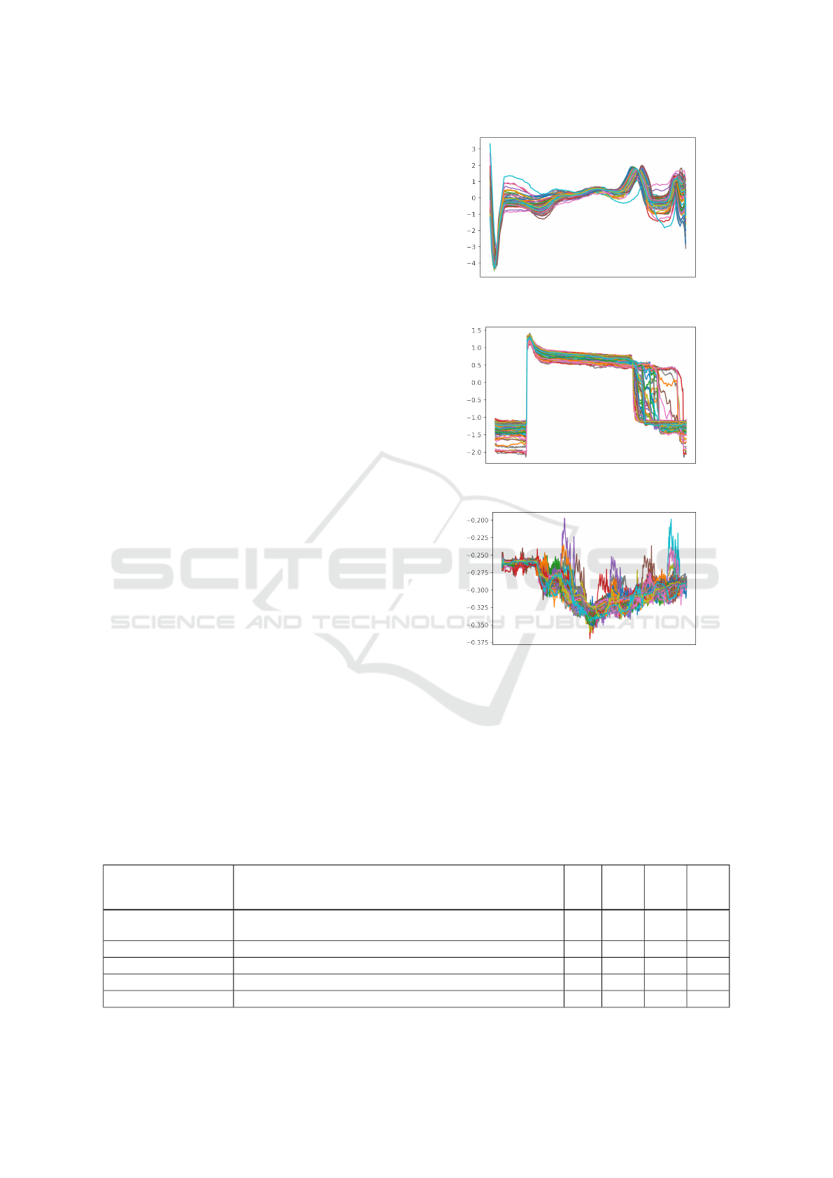
disentanglement. Examples of synthetic time series

sets for datasets ECG5000, FreezerSmallTrain and

InsectEPGSmallTrain are shown in Figures 6, 7 and

The number of additional synthetic time series to

generate per class was calculated as a percentage of

the entire train set size. By doing that, class imbalance

was removed. For example, to create synthetic time

series for each class in the ECG5000 dataset for the

amount equal to 10% of the train set size (500),

Figure 6: 100 generated time series samples for the dataset

ECG5000.

Figure 7: 100 generated time series samples for the dataset

FreezerSmallTrain.

Figure 8: 100 generated time series samples for the dataset

InsectEPGSmallTrain.

variational autoencoders generate 50 synthetic time

series samples per class. For each dataset and train

data combination (either only an original train set,

or an original train set with additional various sized

synthetic sets), we initialized, trained and tested 100

MiniRocket classiﬁer models randomly. Additionally,

1-nearest neighbor (1-NN) classiﬁers, which use

dynamic time warping (DTW) as a distance measure,

Table 2: Time series datasets.

Dataset name Description

Time

series

length

No. of

classes

Train

set size

Test

set size

ECG5000

ECG recordings for ﬁve categorizations of cardiovascular

diseases

140 5 500 4500

FreezerSmallTrain

Power demand of two types of freezers in 20 households 301 2 28 2850

InsectEPGSmallTrain

EPG signals of insect interaction with plants 601 3 17 249

MoteStrain

Distinguishing between humidity and temperature sensors 84 2 20 1252

SmallKitchenAppliances

Electricity consumption of three types of small kitchen appliances 720 3 375 375

ICAART 2022 - 14th International Conference on Agents and Artiﬁcial Intelligence

were trained to observe the effects that synthetic

sets have on simple machine learning classiﬁcation

algorithms. Performance analysis was done by

observing classiﬁcation accuracy, written by (6),

where TP stands for True Positives, TN for True

Negatives, FP for False Positives and FN for False

Negatives in binary classiﬁcation (Hossin and M.N,

2015). The highest achieved test accuracies are shown

in Tables 3 and 4. The bold text marks the highest

test classiﬁcation accuracy of each dataset. The last

two columns represent the maximum positive and

negative differences between the accuracy achieved

with the original train set and the accuracies achieved

with the additional synthetic sets. Each green or

red colored maximum accuracy change represents

whether the dataset’s classiﬁcation accuracies were

improved or degraded by including synthetic time

series samples in the training process. Average test

classiﬁcation accuracies for each dataset, obtained

from training many MiniRocket classiﬁers, using both

original train sets and additional synthetic sets, are

Table 3: Highest time series test classiﬁcation accuracies, obtained with 1-nearest neighbor classiﬁers, which used dynamic

time warping as the distance measure.

Dataset name

Train

Max.

positive

accuracy

change

Max.

negative

accuracy

change

set

Additional synthetic time series samples per class

(% of train set size)

1% 5% 10% 50% 100% 200%

ECG5000

92,44% 92,08% 91,42% 90,77% 89,11% 89,15% 88,53% / -3,91%

FreezerSmallTrain

75,89% 75,89% 75,89% 75,78% 75,64% 75,19% 76,70% +0,81% -0,70%

InsectEPGSmallTrain

100% 100% 100% 100% 100% 100% 100% / /

MoteStrain

83,46% 82,10% 83,46% 83,46% 83,94% 83,94% 82,98% +0,48% -1,36%

SmallKitchenAppliances

64,26% 64,26% 64,26% 64,26% 64,26% 64,26% 64,26% / /

Table 4: Highest time series test classiﬁcation accuracies, obtained with MiniRocket classiﬁers.

Dataset name

Train

Max.

positive

accuracy

change

Max.

negative

accuracy

change

set

Additional synthetic time series samples per class

(% of train set size)

1% 5% 10% 50% 100% 200%

ECG5000

94,08% 94,26% 94,40% 94,17% 93,66% 93,46% 92,93% +0,32% -1,15%

FreezerSmallTrain

94,28% 94,31% 93,15% 93,64% 95,08% 95,50% 93,89% +1,22% -1,13%

InsectEPGSmallTrain

96,38% 96,38% 96,38% 96,38% 96,78% 96,38% 95,98% +0,40% -0,40%

MoteStrain

93,13% 92,33% 92,33% 92,41% 93,29% 92,41% 91,13% +0,16% -2,00%

SmallKitchenAppliances

81,33% 80,00% 78,13% 78,93% 82,13% 76,53% 82,13% +0,80% -4,80%

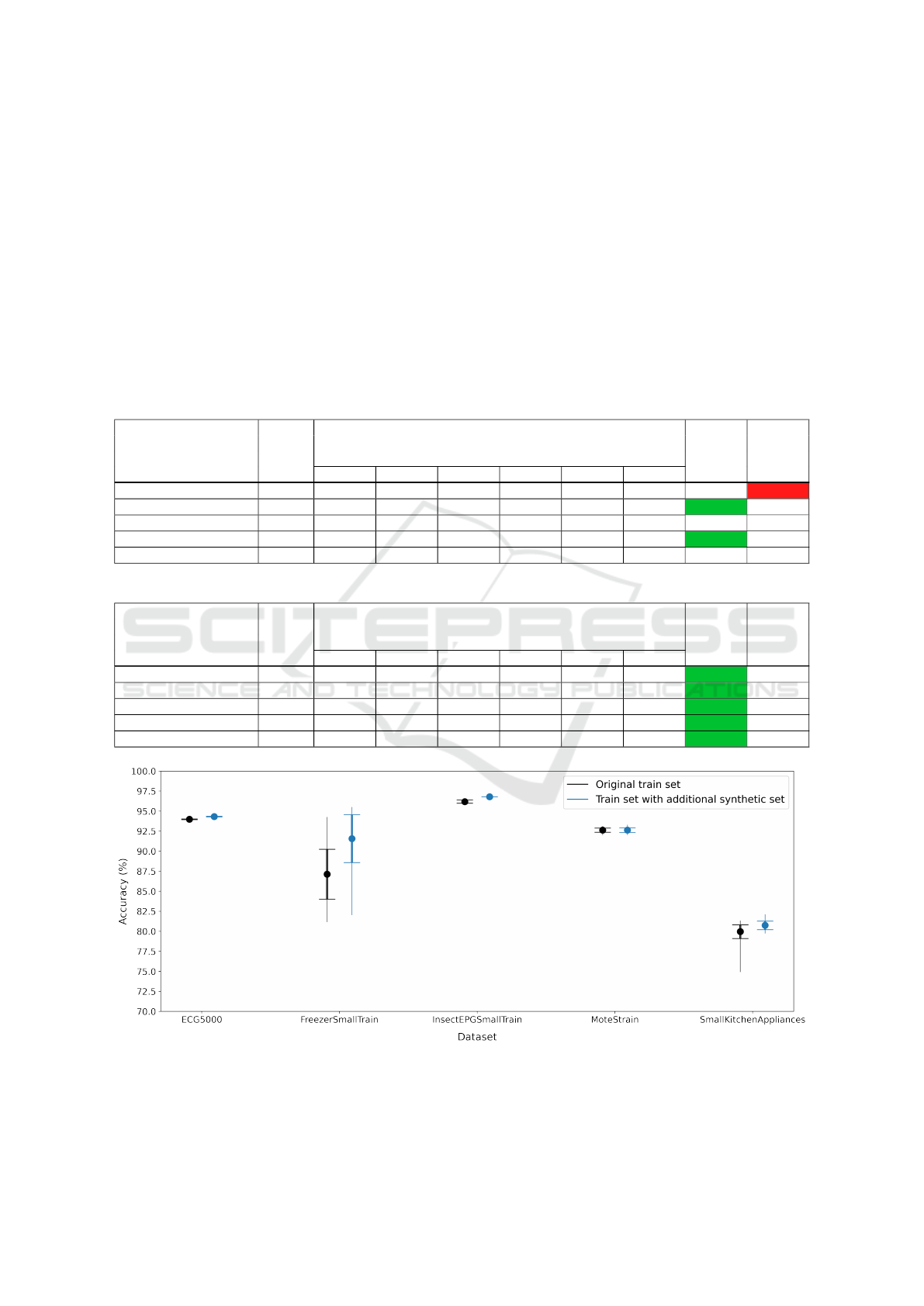
Figure 9: Average test classiﬁcation accuracies, obtained with MiniRocket classiﬁers, which were trained using original train

sets and additional synthetic sets (bold error bars are Standard Deviation, with maximum and minimum accuracies being at

the top and bottom of each line; only the synthetic sets that made the maximum positive accuracy changes, as shown in Table

4, were used for calculating the statistics).

Time Series Augmentation based on Beta-VAE to Improve Classiﬁcation Performance

shown in Figure 9.

Accuracy =

TP + TN

TP + FP + FN + TN

(6)

1-nearest neighbor classiﬁers achieved higher

test accuracies by using additional synthetic time

series samples for the datasets FreezerSmallTrain and

MoteStrain. Synthetic time series samples had no

effect on the classiﬁcation results of the datasets

InsectEPGSmallTrain and SmallKitchenAppliances.

The classiﬁcation accuracies for dataset ECG5000

degraded gradually by increasing the amount of

synthetic time series samples, resulting in a maximum

negative accuracy change of -3,91%.

The MiniRocket classiﬁcation models beneﬁted

from the synthetic time series samples for all

datasets. For the datasets InsectEPGSmallTrain,

MoteStrain and SmallKitchenAppliances, the highest

test classiﬁcation accuracies were achieved with

models trained with additional synthetic sets, which,

for each class, contained an amount of samples equal

to 50% of the train set size. The test accuracies of

trained classiﬁcation models for all datasets, except

SmallKitchenAppliances, decreased when they were

trained with additional synthetic sets, which, for each

class, contained an amount of samples equal to 200%

of the train set size. The test classiﬁcation accuracy

for each dataset could be degraded by training with

a certain amount of synthetic time series samples.

The maximum negative accuracy change of -4,80%

occured for the dataset SmallKitchenAppliances by

training with an additional synthetic set, which, for

each class, contained an amount of samples equal to

100% of the train set size. The maximum positive

accuracy change of 1,22% occured for the dataset

FreezerSmallTrain.

1-nearest neighbor classiﬁers were capable of

classifying all InsectEPGSmallTrain test time series

samples correctly. For all other datasets, MiniRocket

has proven to achieve better classiﬁcation accuracy

results, even up to 18,80% higher compared

to 1-nearest neighbor classiﬁer for the dataset

FreezerSmallTrain. Figure 9 shows that use of a

synthetic set in the training process of the MiniRocket

classiﬁer for the SmallKitchenAppliances dataset

made test accuracies more concentrated towards

the mean classiﬁcation accuracy, yet still achieving

higher maximum accuracy.

5 CONCLUSIONS

A novel augmentation method for generating

synthetic time series with a residual neural network

based variational autoencoder was presented in this

paper. A variational autoencoder, called Beta-VAE,

is trained for each class in a time series classiﬁcation

dataset, and later used for generating synthetic

time series samples. The train set, along with the

synthetic set, were then used for training a time

series classiﬁcation model, MiniRocket. Most of

the highest classiﬁcation accuracies were achieved

with models trained with additional synthetic sets,

which, for each class, contained an amount of

samples equal to 50% of the train set size. Across

the tested datasets, the proposed method achieved

a maximum increase of 1,22% in test classiﬁcation

accuracy in comparison to the baseline results

obtained by training only with original train sets.

An increase of up to 0,81% in the accuracy of

simple machine learning classiﬁers was observed by

benchmarking the proposed augmentation method

with the 1-nearest neighbor algorithm. The amount

of synthetic time series samples should be selected

carefully by trial and error to prevent degradation of

classiﬁcation accuracy. In the future, the proposed

Beta-VAE architecture will be adapted for generating

multivariate time series samples.

ACKNOWLEDGEMENTS

The authors acknowledge the ﬁnancial support from

the Slovenian Research Agency (Research Core

Funding No. P2-0041, as well as Research Projects

No. L7-2633 and No. V2-2117).

REFERENCES

Bagnall, A., Lines, J., Vickers, W., and Keogh, E. (2021).

The uea and ucr time series classiﬁcation repository.

Bank, D., Koenigstein, N., and Giryes, R. (2020).

Autoencoders.

Dempster, A., Schmidt, D., and Webb, G. (2020).

MINIROCKET: A Very Fast (Almost) Deterministic

Transform for Time Series Classiﬁcation.

Gian Antonio, S., Angelo, C., and Matteo, T. (2018).

Chapter 9 - time-series classiﬁcation methods:

Review and applications to power systems data. pages

179–220.

Higgins, I., Matthey, L., Pal, A., Burgess, C. P., Glorot,

X., Botvinick, M., Mohamed, S., and Lerchner, A.

(2017). beta-vae: Learning basic visual concepts with

a constrained variational framework. In ICLR.

Hossin, M. and M.N, S. (2015). A review on

evaluation metrics for data classiﬁcation evaluations.

International Journal of Data Mining and Knowledge

Management Process, 5:01–11.

ICAART 2022 - 14th International Conference on Agents and Artiﬁcial Intelligence

Ismail Fawaz, H., Lucas, B., Forestier, G., Pelletier, C.,

Schmidt, D. F., Weber, J., Webb, G. I., Idoumghar, L.,

Muller, P.-A., and Petitjean, F. (2020). Inceptiontime:

Finding alexnet for time series classiﬁcation. Data

Mining and Knowledge Discovery, 34(6):1936–1962.

Iwana, B. K. and Uchida, S. (2021). An empirical survey of

data augmentation for time series classiﬁcation with

neural networks. PLOS ONE, 16(7):e0254841.

Kingma, D. and Welling, M. (2014). Auto-Encoding

Variational Bayes.

Lines, J., Taylor, S., and Bagnall, A. (2017). Hive-cote:

The hierarchical vote collective of transformation-

based ensembles for time series classiﬁcation. In 2016

IEEE 16th International Conference on Data Mining

(ICDM), pages 1041–1046.

Liu, B., Zhang, Z., and Cui, R. (2020). Efﬁcient

time series augmentation methods. In 2020

13th International Congress on Image and Signal

Processing, BioMedical Engineering and Informatics

(CISP-BMEI), pages 1004–1009.

Liu, W., Li, R., Zheng, M., Karanam, S., Wu, Z., Bhanu, B.,

Radke, R., and Camps, O. (2019). Towards Visually

Explaining Variational Autoencoders.

Middlehurst, M., Large, J., Flynn, M., Lines, J., Bostrom,

A., and Bagnall, A. (2021). HIVE-COTE 2.0: a new

meta ensemble for time series classiﬁcation.

Oh, C., Han, S., and Jeong, J. (2020). Time-series

data augmentation based on interpolation. Procedia

Computer Science, 175:64–71.

Sadati, N., Zafar Nezhad, M., Chinnam, R. B., and Zhu, D.

(2019). Representation Learning with Autoencoders

for Electronic Health Records: A Comparative Study.

Wang, Z., Yan, W., and Oates, T. (2017). Time series

classiﬁcation from scratch with deep neural networks:

A strong baseline.

Time Series Augmentation based on Beta-VAE to Improve Classiﬁcation Performance