
Negative Selection in Classification using DBLOSUM Matrices as
Affinity Function
Adil Ibrahim and Nicholas K. Taylor
Department of Computer Science, Heriot-Watt University, Edinburgh, U.K.
Keywords: Negative Selection, Affinity Function, Distance Measure, BLOSUM, Immune Algorithm, Artificial Immune
Systems.
Abstract: This paper presents a novel affinity function for the Negative Selection based algorithm in binary
classification. The proposed method and its classification performance are compared to several classifiers
using different datasets. One of the binary classification problems includes medical testing to determine if a
patient has a particular disease or not. The DBLOSUM in Negative Selection classifier appears to be best
suited to classification tasks where false negatives pose a major risk, such as in medical screening and
diagnosis. It is more likely than most techniques to result in false positives, but it is as accurate, if not more
accurate than most other techniques.
1 INTRODUCTION
A vital function of the natural immune system is the
release of antibodies to recognize and identify foreign
bodies (antigens), so they can be destroyed or
eliminated. The interaction between the antibody and
the antigen is the basis for the immune response (Qiu
et al., 2015). De Castro and Timmis (de Castro and
Timmis, 2002) describe our body's original cells as
self-sustaining, whereas disease-causing elements are
referred to as nonself-sustaining. The immune system
differentiates between self and nonself patterns with
a process known as self/nonself discrimination. The
natural immune system activity mechanisms and
processes already give rise to a new research direction
in informatics, the artificial immune systems. As
artificial immune systems (AIS) have gained
popularity in a range of uses since 1994 (Forrest et al.
1994), they are now being used in all application
areas, from intrusion to finishing medical diagnosis.
As AIS advances, the choice to use affinity
measurements to describe the strength of the
similarity remains a significant issue. These "affinity
measurements" control the immune system's process
(Raudys et al., 2010).
There needs to be more significant interaction
between immunologists and computer scientists to
develop powerful models that can serve as a basis for
more efficient algorithms (Timmis, 2006).
From the literature review, it is clear that affinity
measures - and recommendations on how to use
them - have not been identified that may be utilized
in classification tasks using AIS, particularly in the
Negative Selection Algorithm (Hamaker and
Boggess, 2004).
This paper introduces a new affinity measure
based on BLOSUM matrix scores in binary
classification using the Negative Selection Algorithm
in medical datasets.
2 THE NEGATIVE SELECTION
ALGORITHM
Artificial immune systems use the Negative Selection
algorithm (NS) as their basic algorithm. Forrest et al.
(1994) proposed and developed the Negative
Selection Algorithm (NS) for detection applications
based on the egative selection principle observed in
the natural immune system. There are two principal
stages to the NS, namely the generation stage and the
detection stage.
Below is the pseudocode of the NS Algorithm as
described and stated by Freitas and Timmis (2007).
The Negative Selection.
Input: a set of “normal” examples (data items), called
self (S)
Ibrahim, A. and Taylor, N.
Negative Selection in Classification using DBLOSUM Matrices as Affinity Function.
DOI: 10.5220/0010771100003116
In Proceedings of the 14th International Conference on Agents and Artificial Intelligence (ICAART 2022) - Volume 3, pages 55-62
ISBN: 978-989-758-547-0; ISSN: 2184-433X
Copyright
c
2022 by SCITEPRESS – Science and Technology Publications, Lda. All rights reserved
55

Output: a set of “mature” T-cells that do not match any
example in S
Repeat
Randomly generate an “immature” T-cell (detector).
Measure the affinity (similarity) between this T-cell
and each example in S.
If the affinity (similarity) between the T-cell and at
least one example in S is greater than a user-defined
threshold hen
Discard this T-cell as a “mature” T-cell.
else
Output this T-cell as a “mature” T-cell.
end if
until stopping criterion.
3 ARTIFICIAL IMMUNE
SYSTEM AND AFFINITY
FUNCTION
Artificial immune systems are solutions-driven
systems using concepts and principles derived from
theoretical immunology and perceived immune
principles, functions and models that are applied to
problem-solving (Raudys et al., 2010) and (Freitas
and Timmis, 2007). When applying immune models,
it is essential to take into account the factors that
contribute to the problem; a suitable affinity function;
and immune algorithms (Raudys et al., 2010)
(Dasgupta, 2006).
In the natural immune system, the antigens (Ag)
represent molecules the immune system must
recognize as nonself. At the same time, antibodies
(Ab) -which are secreted by plasma cells, represent
the proteins that bind to antigens on B-cell
membranes (Raudys et al., 2010). The biological
immune system cannot contain all the antibodies that
could recognize every possible antigen. As a target to
destroying the unknown antigens, the immune
system's plasma cells produce a sequence of
antibodies that become increasingly similar to
unknown antigens. A few examples of AIS antigens
are computer viruses, spam letters, intrusions into
computer systems, and fraud. While antibodies'
detectors example could be a p-dimensional vector
(ab
1
, ab
2
, …, ab
p
) that AIS is trying to make similar
to an antigen vector (ag
1
, ag
2
, …, ag
p
) to be detected
and destroyed (Raudys et al., 2010).
In the natural immune system, affinities between
antigen and different antibodies are the similarities
defined according to p features forming non-covalent
interactions. The affinities in the AIS are similarity
functions based on input features such as r
th
- a
structure that describes antigens and antibodies,
equivalent to Δ
r
= |ag
r
- ab
r
|. An individual function
of the p features composes a distance measure that
could be employed to estimate the similarities, d(ab
i
,
ag
j
) and d(ab
s
, ag
i
), of a particular antigen, Ag
i
, to
different antibodies' detectors Ab
j
and Ab
s
. Similarly,
distances Δ
r
= |ag
r
- ab
r
|, r = 1, 2, …, p, indicate the
degree of similarity between antibodies Ab
i
and Ab
s
(Raudys et al., 2010).
4 THE PROPOSED AFFINITY
FUNCTION
4.1 The BLOSUM Matrix
The Blocks Substitution Matrix (BLOSUM) matrix
scores alignments between diverging evolutionary
protein chains and are often used in bioinformatics.
The BLOSUM matrix, was initially proposed by
Steven and Jorja Henikoff (Henikoff and Henikoff,
1992). They studied blocks of conserved regions of
protein subdivisions with no gaps in the sequence
alignment. The protein sequences that shared similar
percentage identities were gathered into groups and
averaged, which means the higher the similarity, the
closer the evolutionary distance.
The BLOSUM matrix was constructed by
computing the substitution frequencies for all amino
acid pairs. So, each BLOSUM matrix represents a
substitution matrix used to align protein sequences
based on local alignments.
Each score in the BLOSUM matrix reflects one
amino acid's chance to substitute another in a set of
protein multiple sequence alignments. The higher the
score, the more likely the corresponding amino-acid
substitution is.
Equation (1) is used to calculate the score in the
BLOSUM matrix (Henikoff and Henikoff,1992):
𝑠
=
1
𝜆
𝑙𝑜𝑔
𝑞
𝑒
(1)
The numerator (q
ij
) represents the likelihood of the
hypothesis: the two residues i and j are homologous;
hence they are correlated. Thus, q
ij
is the expected
probability or the target frequency of observing
residues i and j aligned in homologous sequence
alignments. The denominator (e
ij
) is the likelihood of
a null hypothesis: the two residues i and j are un-
correlated and unrelated. Hence, they are occurring
independently at their background frequencies. Thus,
e
ij
is the probability expected to observe amino acids
ICAART 2022 - 14th International Conference on Agents and Artificial Intelligence
56

i and j on average in any protein sequence. A scaling
factor 𝜆 is used to convert all terms in the score
matrix to sensible integers. (Eddy, 2004).
4.2 BLOSUM Matrix and Similarity
BLOSUM matrices, as in every scoring scheme, are
based on an overall percentage of sequence similarity
or imply a similarity percentage with increasing
evolutionary divergence. The frequency of matching
residues decreases and vice versa.
Thus, while "Deep" scoring matrices - such as
BLOSUM62 and BLOSUM50 - are effective when
searching long protein domains and target alignments
with 20 to 30% identity. On the other hand, we find
alignments that share 90 to 50% of identity are
targeted by Shallower scoring matrices that are more
effective when searching for such short protein
domains. (Pearson, 2013).
4.3 The DBLOSUM Matrix
Likewise, biological BLOSUM described in
(Henikoff and Henikoff,1992), we define a block of
non-missing values of records, including records
from the two classes, to construct our DBLOSUM
(data-BLOSUM) matrix. We computed initial
alignments by performing multiple alignments,
following the steps described by Henikoff and
Henikoff (Henikoff and Henikoff,1992).
Log Odd Computation: In a given block in the
biological context, all potential amino acid pairs are
counted. Similarly, in our data scenario, the potential
data-item pairs are the data items in the same column.
So, for each column, a total of all data items is
counted. After these counts have been computed, they
are utilised to determine a matrix Q in which an item
q
ij
represents the frequency with which items i and j
appear in various columns in the block.
From the quantity mentioned above, the
likelihood of the appearance of the i-th entry is
calculated using (2).
𝑝
=𝑞
𝑞
2
(2)
Then, following (Henikoff and Henikoff,1992), the
expected likelihood, e
ij
, of appearance for each i, j
pair can be estimated using (3).
𝑒
=
𝑝
𝑝
,𝑖=
𝑗
2𝑝
𝑝
,𝑖≠
𝑗
(3)
Finally, we compute an odd log ratio using (4) below:
𝑟
=𝑙𝑜𝑔
𝑞
𝑒
(4)
The odd log-ratio, 𝑟
, calculated in (4) appears in a
generic entry in our DBLOSUM matrix. An intuitive
interpretation for this generic form is as follows:
When the observed rates are as expected or more than
expected, 𝑟
≥ 0, and when the observed rates are
lower than expected, such as a rare mutation in amino
acids, 𝑟
< 0.
4.4 Classification and the DBLOSUM
Matrices
The binary classification model under investigation
uses DBLOSUM matrices in the classification
process. The DBLOSUM matrix is constructed from
dataset values following the original BLOSUM
matrix calculations described in the previous section.
The training set extracted from a dataset is the
block that is used to generate the DBLOSUM matrix.
Three matrices will be generated in each binary
classification test: A self DBLOSUM matrix
generated from one class, a nonself DBLOSUM
matrix generated from the other class, and a combined
DBLOSUM from the whole training set combining
the two classes.
4.5 DBLOSUM Scores
A negative score in the BLOSUM matrix indicates
that the alignment of two amino acids in a database
occurred less frequently than by chance. Zero scores
in the BLOSUM matrix indicate that the rate at which
the pair of amino acids were aligned in a database was
just presumed by chance. In contrast, a positive score
means that the alignment occurred more often than
just by chance. This scoring mechanism represents an
essential feature in the learning process of our binary
classification model.
In the proposed DBLOSUM matrix, a positive or
higher score of a given two data items infers that these
two values are likely to appear in the same class, and
a negative or low score proposes that these two values
are unlikely to be in the same class. At the same time,
and similar to the BLSOUM scoring mechanism, a
zero score in our DBLOSUM matrix indicates that the
pair of the data items occurred just by chance.
The score in the DBLOSUM is the primary
learning point in our binary classification model.
Each score in the DBLOSUM matrix tells how each
pair of values within the training set are related.
Negative Selection in Classification using DBLOSUM Matrices as Affinity Function
57
Through the DBLOSUM scores, we are trying to
discover hidden patterns in the dataset to be classified.
5 THE CLASSIFICATION
MODEL
Our binary classification model uses DBLOSUM
matrices in the classification process. The
DBLOSUM matrix is constructed from dataset values
following the original BLOSUM matrix calculations
and described in 4.3.
The training set extracted from a dataset is the
block that is used to generate the DBLOSUM matrix.
Three matrices will be generated in each binary
classification test: A self DBLOSUM matrix
generated from one class, a nonself DBLOSUM
matrix generated from the other class, and a combined
DBLOSUM from the whole training set combining
the two classes.
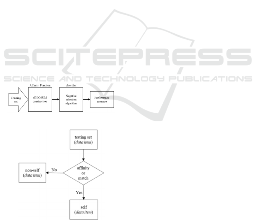
Fig. 1 shows the classification model using the
DBLOSUM matrices as an affinity function in the
Negative Selection Algorithm. Our binary
classification model uses the DBLOSUM matrices
constructed from the dataset to be classified. The
scores in the DBLOSUM matrices are then used as
affinity function in the Negative Selection Algorithm.
Fig. 2 shows classification processes based on the
Negative Selection algorithm and the concept of
self/nonself discrimination.
Figure 1: The basic model involved in this study.
Figure 2: The rule to generate detectors in the Negative
Selection Algorithm is used for the classification.
5.1 Learning Process
Our model explores the hidden pattern amongst data
in a dataset similar to discovering and exploring the
evolutionary distance or divergence between proteins
using the scoring scheme matrix.
Each DBLOSUM score value is a key learning
point in discovering the relationships between pair
values within the training set. The process of
discovering the relationships between pair values
covers either all pairs in the training set, i.e. 0%
similarity and all records are involved in the process
or covers pairs values in a block of records within the
training set that shares a specific similarity
percentage.
The same as the similarity in the original
BLOSUM matrix works, the noisier the data is, the
more challenging it to discover the hidden patterns.
Hence, the lowest similarity or the 0% similarity
would be the best to use because it includes all the
training set records. In contrast, high DBLOSUM
similarity can be used with less noisy data;
nevertheless, increasing the similarity percentages
may be hindered by the possibilities of lacking paired
values, leading to unpaired matrices. Missing scores
are treated the same as missing data items; all are set
to zero.
The learning process finishes after exploring the
relationships between all pairs of values in the
selected block and calculate the associated scores that
define the relationships between each pair of values
in the selected block.
5.2 The Classification Process
The generated DBLOSUM is used in the
classification process. Seed values - usually from the
last row in the testing set- are paired with their
corresponding features values in the first row of the
testing set, then a look-up process finds the relevant
score of the paired value from the DBLOSUM matrix.
The DBLOSUM score tells whether the pair values
are self or nonself (see Fig. 2) - or in other words, the
pair values belong to the same class or not. Values in
the first row then become seed values for their
corresponding features in the second row, and the
process continues in pairing corresponding values
row by row.
So, to classify a record B = b
1
, b
2
, . . ., b
n
, we use
the seed values that make the previous raw, say record
A = a
1
, a
2
, . . ., a
n
. The pairs (a
i
,b
i
) are passed into the
Negative Selection Algorithm using their
calculated DBLOSUM score s(a
i
,b
i
) as matching
function. If the DBLOSUM scores(a
i
,b
i
) ≥ threshold
ICAART 2022 - 14th International Conference on Agents and Artificial Intelligence
58

then mark b
i
a self data item, i.e. the value b
i
belong
to the same class as a
i
, otherwise b
i
is marked a
nonself value or in other words, b
i
belong to the other
class in the dataset.
Finally, the record B is classified based on the
following rule:
if
𝑏
≥ 𝑡ℎ𝑟𝑒𝑠ℎ𝑜𝑙𝑑
then
B = self record; A and B are in the same class.
else
B = nonself record; A and B are not in the same class.
6 THE EXPERIMENTS
The proposed classification model in Fig. 1 has been
implemented using the DBLOSUM matrices as an
affinity function in the Negative Selection Algorithm
(NS). As Fig. 2 shows, no detectors were generated in
all experiments; instead, we have used the rules of
generating the detectors directly in the classification
process.
We have used three datasets to test our
classification model, including the Wisconsin Breast
cancer dataset, Pima Indians Diabetes Database, and
Adult income dataset.
The data in each dataset has been thoroughly
studied, and basic statistics have been calculated
before running the experiments. Nevertheless, we did
not include any of the basic statistics in the
experiments. Real values were used in the
classification process.
We have divided the dataset under classification
into two sets, training and testing sets in each
experiment. The training set in each experiment is no
more than two-thirds of the total records in the
dataset. Missing values were treated as a zero.
We construct the self-DBLOSUM, nonself-
DBLOSUM, and combined DBLOSUM matrices
using the same training set as explained in section 4.4.
Missing scores are treated as a zero.
Implementing the classification as detailed in 5.2, we
have found that the DBLOSUM score supplies
enough information to verify whether a pair of data
items taken from the same feature in a dataset belongs
to the same class or not. We then completed the
classifications using the rule in section 5.2.
7 RESULTS
To describe the performance of the proposed model,
we used the confusion matrix. As shown below, true-
positive, true-negative, false-positive, and false-
negative counts are represented by TP, TN, FP, and
FN. To test the true-positive rate and the true-negative
rate, we use the sensitivity and specificity calculated
by (5) and (6), respectively.
𝑠𝑒𝑛𝑠𝑖𝑡𝑖𝑣𝑖𝑡𝑦 =
𝑇𝑃
𝑇𝑃
+
𝑇𝑁
(5)
𝑠𝑝𝑒𝑐𝑖𝑓𝑖𝑐𝑖𝑡𝑦 =
𝑇𝑁
𝑇𝑁
+
𝐹𝑃
(6)
We have also determined the effectiveness of the
proposed model by using the most common empirical
measure, accuracy, by using (7):
𝑎𝑐𝑐𝑢𝑟𝑎𝑐𝑦 =
𝑇𝑃 +𝑇𝑁
𝑇𝑃+𝑇𝑁+𝐹𝑃+𝐹𝑁
(7)
Equation (8) is used to calculate precision, and to
test the obtained accuracy, we have used the F-
measure calculated in (9).
𝑝𝑟𝑒𝑐𝑖𝑠𝑖𝑜𝑛 =
𝑇𝑃
𝑇𝑃
+
𝐹𝑃
(8)
𝐹1 = 2×
𝑝𝑟𝑒𝑐𝑖𝑠𝑖𝑜𝑛×𝑠𝑒𝑛𝑠𝑖𝑡𝑖𝑣𝑖𝑡𝑦
𝑝
𝑟𝑒𝑐𝑖𝑠𝑖𝑜𝑛+𝑠𝑒𝑛𝑠𝑖𝑡𝑖𝑣𝑖𝑡
𝑦
(9)
We have run experiments on three -different-
datasets from different domains. Table 1 shows a
brief description of each dataset.
Table 1: Datasets details.
Dataset
Number
of
instances
Involved
attributes
Characteristics
Missing
values
Classification
self Nonself
Breast cancer 699 9 Multivariate. Integers Yes Benign Malignant
Pima Indians diabetes 768 8 Multivariate. Integers, real Yes negative positive
Adult Income 48,842 14 Multivariate. Integers, categorical Yes <= 50K > 50K
Negative Selection in Classification using DBLOSUM Matrices as Affinity Function
59
The following sections detail the obtained results
in each dataset.
7.1 Wisconsin Breast Cancer Dataset
The Wisconsin Breast Cancer dataset (Mangasarian
and Wolberg, 1990) (Mangasarian et al., 1990) has
two classes: benign and malignant. There are 699
instances in it, 65.5% is Benign (self class), and
34.5% is Malignant (nonself class).
The block of the training set is made of 10%
similarity. The DBLOSUM matrix used is the Self-
DBLOSUM matrix.
With the default threshold value t = 0, the
accuracy obtained is 97.14%. Table 2 shows the
performance evaluation metrics among the
classifiers. Fig. 3 shows a comparison based on the
accuracy, sensitivity, and specificity of these different
classifiers against our proposed model.
According to (Ed-daoudy and Maalmi, 2020), an
average accuracy of 94.85% was obtained for
Decision Tree (DT) (J48), 96.42% for Random Forest
(RF), 96.85% for Logistic Regression (LG), 97.42%
for Bayes Net (BN), 97.00% for SVM, and 95.57%
for Multilayer Perceptron (ANN).
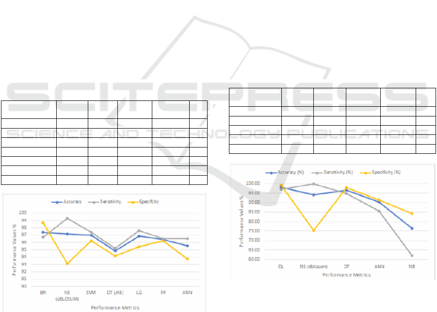
Table 2: Breast cancer performances evaluation metrics.
Classifiers
Accuracy
(%)
Precision
(%)
Sensitivity
(%)
Specificity
(%)
F1
score
BN 97.42 99.33 96.72 98.75 98.01
NS-DBLOSUM 97.14 96.45 99.27 93.12 97.84
SVM 97.00 98.02 97.38 96.26 97.70
DT(J48) 94.85 96.89 95.20 94.19 96.04
LG 96.85 97.60 97.60 95.43 97.60
RF 96.42 98.00 96.51 96.26 97.25
ANN 95.57 96.72 96.51 93.77 96.61
Figure 3: Accuracy, sensitivity, and specificity for the
Breast cancer dataset.
7.2 Pima Indians Diabetes Dataset
The diabetes dataset has two classes, which
represents those who are tested negative and positive.
The tested negative class (self class) is 65.1%, and the
tested positive class (nonself class) is 34.9%.
The block of the training set is made of 0%
similarity. Each class is represented with 50%,
records in the block were selected randomly. The
DBLOSUM matrix used is the combined DBLOSUM
generated from the training set.
With the default threshold value t = 0. The
accuracy obtained is 94.10%. Table 3 shows the
performance evaluation metrics among other
classifiers. Fig. 4 shows a comparison based on the
accuracy, sensitivity, and specificity of these different
classifiers against our proposed model.
7.3 Adult Income Dataset
The Adult Income dataset, which can be found in the
University of California Irvine (UCI) Machine
Learning Repository (Dua and Graff, 2019), includes
data on 48,842 different instances spanning 14
different attributes. Among them are six continuous
and eight categorical attributes. The Adult Income
dataset covers the information of individuals from 42
Table 3: Pima Indians diabetes performances evaluation
metrics.
Classifiers
Accuracy
(%)
Precision
(%)
Sensitivity
(%)
Specificity
(%)
F1
score
DL 98.07 95.22 96.99 99.29 96.81
NS-DBLOSU
M
94.10 92.81 100.00 75.31 96.27
DT 96.62 94.02 94.74 97.86 94.72
ANN 90.34 88.05 85.58 91.43 85.98
BN 76.33 59.07 62.11 84.29 61.67
Figure 4: Accuracy, sensitivity, and specificity for the Pima
Indians diabetes dataset.
different nations. The collected data include the
person's age, working-class, education, marital status,
occupation, relationship within a family, race, gender,
capital gain and loss, the number of hours worked per
week and the person's native country. Based on the
given set of attributes in the Adult Income dataset, the
ICAART 2022 - 14th International Conference on Agents and Artificial Intelligence
60

class attribute indicates whether a person earns more
than 50 thousand Dollars per year or not.
The Adult income dataset has imbalanced data. It has
76% for those who earn ≤ 50K and 24% for those who
earn > 50K. To reduce the bias resulting from the
imbalance between the two classes, the records in the
training set block we used consists of 50% from each
class; records were selected randomly. The proposed
model has achieved 87.69% accuracy using both self
and the nonself DBLOSUM matrices with 0%
similarity. Table 4 shows the classification results of
the proposed model against previously obtained
results reported in (Chakrabarty and Biswas, 2018),
including the Hyper-Parameter-Tuned Gradient
Boosting Classifier (HPTGBC), the PCA with
Support Vector Machine (PCA+SVM), the Gradient
Boosting Classifier (GBC), and the XGBOOST
classifier. Fig. 5 shows the proposed model's
accuracy, sensitivity, and specificity against these
classifiers.
Table 4: Adult income performances evaluation metrics.
Classifiers
Accuracy
(%)
Precision
(%)
Sensitivity
(%)
Specificity
(%)
F1
score
HPTGBC 88.16 88.00 88.00 X 88.00
NS-DBLOSUM 87.69 95.13 91.12 53.62 93.00
PCA+SVM 84.92 x x x x
GBC 86.92 x x x x
XGBOOST 87.53 x x x x
Figure 5: Accuracy, sensitivity, and specificity for the Adult
income dataset.
8 DISCUSSION
From Fig. 3, it is clear that the DBLOSUM model has
achieved the highest sensitivity (99.27%) compared
to BN (96.72%), SVM (97.38%), DT(J48) (95.20%),
LG (97.60%), RF (96.51%), and ANN (96.51%)
classifiers with the breast cancer dataset. The high
sensitivity of the DBLOSUM model helps correctly
diagnose malignancy in the breast cancer dataset
compared to all other classifiers. Moreover, the
model's accuracy of 97.14% comes second after the
BN accuracy (97.42%) – see Table 2; this puts its
accuracy ahead of the other five classifiers with this
dataset. However, when using the breast cancer
dataset, we find that the DBLOSUM model has the
lowest specificity (93.12%) compared to the other
classifiers using the same dataset; this increases the
rate of false positives of the model compared to the
other classifiers using the dataset. Similarly, when
using the diabetes dataset and as shown in Fig. 4, the
DBLOSUM model manages a sensitivity of 100%
against the DL (96.99%), DT (94.74%), ANN
(85.58%), and BN (62.11%) classifiers – see Table 3.
The sensitivity achieved by the model in the diabetes
dataset means that it is the best classifier to correctly
diagnose diabetes. Again, the model has the lowest
specificity on the diabetes dataset. However, it
maintains a good accuracy of 94.10% among the
classifiers using this dataset. The DBLOSUM model
achieved an accuracy of 87.69% using the adult
income dataset, just below the HPTGBC classifier
(88.16%); this is better than the accuracy obtained by
XGBOOST (87.53%), GBC (86.29%), and the
PCA+SVM (84.92%) classifiers using the same
dataset. The model again delivers the highest
sensitivity of 91.12% against the sensitivity of the
HPTGBC classifier (88.00%).
9 CONCLUSIONS
In this paper, the performance of the Negative
Selection classifier was tested using the DBLOSUM
as an affinity function in three different datasets;
Wisconsin Breast Cancer, Pima Indians Diabetes and
Adult Income datasets.
The obtained results were compared to six
different classifiers that have previously used the
Wisconsin Breast Cancer dataset. The model
achieved the highest sensitivity of 99.27% compared
to all other classifiers. The best accuracy obtained
was 97.14%, second after the BN accuracy (97.42%)
and higher than SVM (94.00%), DT(J48) (94.85%),
LG (96.85%), RF (96.42%), and ANN (95.57%).
The same method was also compared against four
classifiers that have previously used the Pima Indians
Diabetes dataset, with a 100.00% sensitivity, the
model's best accuracy was 94.10%. The obtained
accuracy is the third after the DL (98.07%) and DT
(96.62%) classifiers and higher than the ANN
(90.34%) and BN (76.33%) classifiers.
The performance was also tested against another
four classifiers that have previously used the Adult
Income dataset. The best accuracy obtained was
Negative Selection in Classification using DBLOSUM Matrices as Affinity Function
61

87.69%, the second-best accuracy after the HPTGBC
classifier (88.16%).
The models’ accuracy is better than the
PCA+SVM (84.92%), GBC (86.92%), and
XGBOOST (87.53%).
The DBLOSUM in Negative Selection classifier
appears to be best suited to classification tasks where
false negatives pose a major risk, such as in medical
screening and diagnosis. It is more likely than most
techniques to result in false positives, but it is as
accurate, if not more accurate than most other
techniques.
ACKNOWLEDGEMENTS
This work was supported in part by a bursary from the
Prisoners of Conscience Appeal Fund and in part by
a scholarship from Heriot-Watt University, UK.
We thank the Department of Computer Science at
the University of Wisconsin - Madison, USA, for the
opportunity to attend talks, seminars, and discussions
in the field of AI and ML.
The Breast Cancer database was obtained from
the University of Wisconsin Hospitals, Madison,
from Dr William H. Wolberg. The Pima Indians
Diabetes and Adult Income datasets can be accessed
from the Machine Learning Repository at the
University of California, Irvine.
REFERENCES
Chakrabarty, N. and Biswas, S. (2018). A statistical
approach to adult census income level prediction. In
2018 International Conference on Advances in
Computing, Communication Control and Networking
(ICACCCN), pages 207–212. IEEE.
Dasgupta, D. (2006). Advances in artificial immune
systems. In IEEE computational intelligence magazine.
IEEE.
de Castro, L. N. and Timmis, J. (2002). Artificial immune
systems: A novel approach to pattern recognition. In
Artificial Neural Network in Pattern Recognition.
University of Paisley.
Dua, D. and Graff, C. (2019). UCI machine learning repos-
itory
Ed-daoudy, A. and Maalmi, K. (2020). Breast cancer
classification with reduced feature set using association
rules and support vector machine. In Network Modeling
Analysis in Health Informatics and Bioinformatics,
volume 9, pages 1–10. Springer.
Eddy, S. R. (2004). Where did the blosum62 alignment
score matrix come from? In Nature biotechnology,
volume 22, pages 1035–1036. Nature Publishing
Group.
Forrest, S., Perelson, A., Allen, L., and Cherukuri, R.
(1994). Self-nonself discrimination in a computer. In
Proceedings of 1994 IEEE Computer Society
Symposium on Research in Security and Privacy. IEEE
Comput. Soc. Press.
Freitas, A. and Timmis, J. (2007). Revisiting the
foundations of artificial immune systems for data
mining. In IEEE transactions on evolutionary
computation. IEEE.
Hamaker, J. and Boggess, L. (2004). Non-euclidean
distance measures in airs, an artificial immune
classification system. In Proceedings of the 2004
Congress on Evolutionary Computation (IEEE
Cat.No.04TH8753). IEEE.
Henikoff, S. and Henikoff, J. G. (1992). Amino acid
substitution matrices from protein blocks. In
Proceedings of the National Academy of Sciences -
PNAS, volume 89, pages 10915–10919,
WASHINGTON. National Academy of Sciences of the
United States of America.
Mangasarian, O. L., Setiono, R., and Wolberg, W. H.
(1990). Pattern recognition via linear programming:
Theory and application to medical diagnosis. In Large-
Scale Numerical Optimization, pages 22–30. SIAM
Publications.
Mangasarian, O. L. and Wolberg, W. H. (1990). Cancer
diagnosis via linear programming. Technical report,
University of Wisconsin-Madison Department of
Computer Sciences.
Pearson, W. R. (2013). Selecting the right similarity-
scoring matrix. In Current protocols in bioinformatics,
volume 43, pages 3–5. Wiley Online Library.
Qiu, T., Xiao, H., Qingchen, Z., Qiu, J., Yang, Y., Wu, D.,
Cao, Z., and Zhu, R. (2015). Proteochemo-metric
modeling of the antigen-antibody interaction: New
fingerprints for antigen, antibody and epitope-paratope
interaction. In PloS one. doi = 10.1371/jour-
nal.pone.0122416.
Raudys, S., Arasimavicius, J., and Biziuleviciene, G.
(2010). Learning the affinity measure in real and
artificial immune systems. In 2010 3rd International
Conference on Biomedical Engineering and
Informatics. IEEE.
Timmis, J. (2006). Challenges for artificial immune
systems. In Neural Nets. Springer Berlin Heidelberg.
ICAART 2022 - 14th International Conference on Agents and Artificial Intelligence
62
