NeuralQAAD: An Efﬁcient Differentiable Framework for Compressing

High Resolution Consistent Point Clouds Datasets

Nicolas Wagner and Ulrich Schwanecke

RheinMain University of Applied Sciences, Wiesbaden, Germany

Keywords:

Point Clouds, Compression, Deep Learning.

Abstract:

In this paper, we propose NeuralQAAD, a differentiable point cloud compression framework that is fast,

robust to sampling, and applicable to consistent shapes with high detail resolution. Previous work that is able

to handle complex and non-smooth topologies is hardly scaleable to more than just a few thousand points. We

tackle the task with a novel neural network architecture characterized by weight sharing and autodecoding.

Our architecture uses parameters far more efﬁciently than previous work, allowing it to be deeper and more

scalable. We also show that the currently only tractable training criterion for point cloud compression, the

Chamfer distance, performances poorly for high resolutions. To overcome this issue, we pair our architecture

with a new training procedure based on a quadratic assignment problem. This procedure acts as a surrogate loss

and allows to implicitly minimize the more expressive Earth Movers Distance (EMD) even for point clouds

with way more than 10

points. As directly evaluating the EMD on high resolution point clouds is intractable,

we propose a new divide-and-conquer approach based on k-d trees, which we call EM-kD. The EM-kD is

shown to be a scaleable and fast but still reliable upper bound for the EMD. NeuralQAAD demonstrates on

three datasets (COMA, D-FAUST and Skulls) that it signiﬁcantly outperforms the current state-of-the-art both

visually and qualitatively in terms of EM-kD.

1 INTRODUCTION

In recent years, deep learning has been successfully

applied to numerous computer vision and graphics

tasks, such as classiﬁcation, segmentation, or com-

pression. However, most progress has been achieved

in the 2D domain based on the regular data struc-

ture of images. Unfortunately, the same methods

cannot easily be generalized to unstructured three-di-

mensional data. Memory consumption and computa-

tional cost usually increase rapidly in 3D, which lim-

its the applicability of GPU-accelerated algorithms.

In particular, gradient descent algorithms suffer from

this phenomenon. Especially irregular representa-

tions such as point clouds or meshes are only sparely

covered so far. However, as the typical output of 3D

scanners, high resolution point clouds are widely used

in autonomous driving, robotics, and other domains

to represent surfaces or volumes. A tool capable of

reducing the memory requirements of point clouds

that can be added to a differential pipeline is therefore

highly desirable. Unfortunately, point clouds pose a

particular challenge since points may not only be ir-

regularly but also sparsely scattered in space and, in

contrast to meshes, do not provide explicit neighbor-

hood information. Furthermore, the habit of neural

networks to generate smooth signals seems to hin-

der the reconstruction of high frequencies, complex

topologies, and discontinuities.

The current state-of-the-art in differentiable point

cloud compression mainly focuses on the idea of

folding one or multiple ﬁxed input manifolds into a

target manifold (Chen et al., 2020; Groueix et al.,

2018; Deprelle et al., 2019). Regardless of the re-

spective concept, the size of the point clouds that

can be processed by current hardware is very limited,

since mainly pointwise neural networks are used. Re-

cently, sampling techniques have been used to over-

come this problem (see e.g. (Mescheder et al., 2019;

Groueix et al., 2018; Deprelle et al., 2019)). Thereby,

the difference between two point clouds is usually

measured using the Chamfer distance (see e.g. (Chen

et al., 2020; Groueix et al., 2018; Zhao et al., 2019)).

The popularity of the Chamfer distance stems from

its ability to measure the distance from a point in

one point cloud to its nearest neighbor in the other

and vice versa. However, using the Chamfer metric

on point cloud samples badly misguides gradient de-

Wagner, N. and Schwanecke, U.

NeuralQAAD: An Efﬁcient Differentiable Framework for Compressing High Resolution Consistent Point Clouds Datasets.

DOI: 10.5220/0010772500003124

In Proceedings of the 17th International Joint Conference on Computer Vision, Imaging and Computer Graphics Theory and Applications (VISIGRAPP 2022) - Volume 4: VISAPP, pages

811-822

ISBN: 978-989-758-555-5; ISSN: 2184-4321

811

scent optimization algorithms. This is due to the fact

that not all points are considered when determining

the nearest neighbors of point cloud samples. There-

fore, with high probability, distances between false

matches are minimized. However, although a local

optimum can be achieved, high frequencies are usu-

ally lost as a result. This problem is particularly se-

vere when a point cloud is densely sampled and con-

tains detailed, ﬁne structures. The most commonly

used PointNet encoders (Chen et al., 2020; Groueix

et al., 2018; Zhao et al., 2019) suffer from exactly this

problem as they rely on lossy global pooling layers

that can only be generalized to a limited extent. Even

worse, the Chamfer distance is generally known as an

unsuitable criterion for the similarity of point clouds

(Liu et al., 2020; Achlioptas et al., 2018). The earth

movers distance (EMD), that solves a linear assign-

ment problem (LAP) between compared point clouds,

is considered to be more appropriate (Liu et al., 2020;

Achlioptas et al., 2018). However, solving a linear as-

signment problem has a cubic running time for an ex-

act solution and even approximations are not efﬁcient

enough for training neural networks on point clouds

with more than a few thousand points.

In this paper we present NeuralQAAD, a deep au-

todecoder for compact representation of high resolu-

tion point cloud datasets. NeuralQAAD is based on

a speciﬁc neural network architecture that overlays

multiple foldings deﬁned on learned and shared fea-

tures to reconstruct point clouds. Our main contribu-

tions are

1. a new scaleable point cloud autodecoder architec-

ture that is able to efﬁciently recover high resolu-

tion consistent shapes,

2. training algorithms that are motivated by a newly

deﬁned quadratic assignment problem (QAP),

3. a validation that our approach outperforms the

current state-of-the-art on high resolution point

clouds, and ﬁnally

4. a novel dataset of detailed skull CT-scans.

2 RELATED WORK

In the following, we give a brief overview of the three

main areas of related work: 1. algorithms and data

structures to process point clouds using deep learning,

2. neural network architectures for compressing point

clouds, and 3. assignment problems.

2.1 Deep Learning for 3D Point Clouds

Various data structures for representing 3D data in the

context of deep learning have been examined, includ-

ing meshes (Bruna et al., 2014), voxels (Wang et al.,

2018; Maturana and Scherer, 2015), multi-view (Su

et al., 2015), classiﬁer space (Mescheder et al., 2019)

and point clouds (Qi et al., 2017a). Point clouds are

often the raw output of 3D scanners and are char-

acterized by irregularity, sparsity, missing neighbor-

hood information, and permutation invariance. To

cope with these challenges, many approaches convert

point clouds into other representations such as dis-

crete grids or polygonal meshes.

Nonetheless, each data structure comes with its

downsides. Voxelization of point clouds (Girdhar

et al., 2016; Sharma et al., 2016; Wu et al., 2016;

Roveri et al., 2018) enables the use of convolutional

neural networks but sacriﬁces sparsity. This leads

to signiﬁcantly increased memory consumption and

decreased resolution. Utilizing meshes requires to

reconstruct neighborhood information. This can ei-

ther be done handcrafted, with the risk of wrongly

introducing a bias, or learned for a particular task

(Chen et al., 2020). In both cases, again, memory

consumption increases signiﬁcantly due to the stor-

age of graph structures. Related to the transforma-

tion into meshes are approaches that deﬁne convo-

lution directly on point clouds (Tatarchenko et al.,

2018; Xu et al., 2018). Another approach is to em-

bed point clouds into a classiﬁer space via fully con-

nected neural networks (Mescheder et al., 2019; Park

et al., 2019). However, this approach does not take

into account the advantages of point clouds, as neu-

ral networks tend to smooth the irregularity of point

clouds and thus may miss detailed structures. Also,

these methods are not trainable out of the box, as a

countable ﬁnite (point) set must be deﬁned on an un-

countable space.

PointNet (Qi et al., 2017a) was the ﬁrst neural net-

work to directly work on point clouds. It applies a

pointwise fully connected neural network to extract

pointwise features that are combined by max-pooling

to create global features. Thus, all the previously

mentioned disadvantages apply to PointNet. There is

numerous work on extending PointNet to be sensitive

to local structures (see e.g. (Qi et al., 2017b; Zhou

and Tuzel, 2018)). In this paper, we focus on unsuper-

vised learning. Most of the aforementioned methods

are only applicable in a supervised setting. We de-

ploy PointNet to produce intermediate encodings but

discard it for the ﬁnal compression.

VISAPP 2022 - 17th International Conference on Computer Vision Theory and Applications

812

2.2 Deep Point Cloud Compression

An autoencoder is the standard technique when it

comes to compressing data using deep learning. How-

ever, recent work (Park et al., 2019) demonstrates

that solely utilizing a decoder can be sufﬁcient, at

least in the 3D domain. Here, the encoder is re-

placed by a trainable latent tensor. Deep generative

models like generative adversarial networks (GANs)

(Goodfellow et al., 2014) or variational autoencoders

(VAEs) (Kingma and Welling, 2014) can also be ap-

plied to reduce dimensionality. But they add over-

head complexity and are rarely used for this purpose,

although for VAEs (Zadeh et al., 2019) it may be suf-

ﬁcient to train only one decoding part, just like for

standard autoencoders.

Most commonly, deep learning based compres-

sion methods for 3D point clouds either rely on vox-

elization (Girdhar et al., 2016; Sharma et al., 2016;

Wu et al., 2016) or have one neuron per point in a fully

connected output layer (Fan et al., 2017; Achlioptas

et al., 2018). The latter approaches are hardly train-

able for large-scale point clouds and require a huge

number of parameters even for small point clouds. In

contrast, FoldingNet (Yang et al., 2018) and Fold-

ingNet++ (Chen et al., 2020) rely on PointNet for

encoding and use pointwise decoders that are based

on the folding concept. Thereby folding describes

the process of transforming a ﬁxed input point cloud

to a target point cloud by a pointwise neural net-

work. FoldingNet++ additionally learns graph struc-

tures for localized transformations partly avoiding

the problem of the smooth signal bias. Another ap-

proach based on the concept of folding is AtlasNet

(Groueix et al., 2018), which folds and translates mul-

tiple 2D patches to cover a target surface. The exten-

sion AtlasNetV2 (Deprelle et al., 2019) makes these

patches trainable. AtlasNet and AtlasNetV2 suffer

from the problem that they are hardly scalable and

sometimes fail to glue all patches together without

artifacts. Other pointwise autoencoders include 3D

Point Capsule Networks (Zhao et al., 2019), which

use multiple latent vectors per instance to capture dif-

ferent basis functions while using a dynamic routing

scheme (Sabour et al., 2017).

All of the state-of-the-art point cloud autoen-

coders (Chen et al., 2020; Groueix et al., 2018; Zhao

et al., 2019) are trained by optimizing the Chamfer

distance. Older approaches such as (Fan et al., 2017;

Achlioptas et al., 2018) trained on the earth mover

distance, as well, but are restricted in point cloud size.

In this work, we provide a surrogate loss for minimiz-

ing the EMD even for high resolution point clouds.

2.3 Assignment Problems

In its most general form, an assignment problem con-

sists of several agents and several tasks. The goal is

to ﬁnd an assignment from the agents to the tasks that

minimizes some cost function. The term assignment

problem is often used as a synonym for the linear as-

signment problem (LAP). LAPs have the same num-

ber of agents and tasks. The cost function is deﬁned

on all assignment pairs. Kuhn proposed a polynomial

time algorithm, known as the Hungarian algorithm

(Kuhn, 1955), that can solve a LAP in quartic runtime.

Later algorithms such as (Edmonds and Karp, 1972)

or (Jonker and Volgenant, 1986) improved to cubic

runtime. A fast and parallelizable ε-approximation

algorithm (the auction algorithm) to determine an al-

most optimal assignment was introduced in (Bert-

sekas, 1988) and used in (Fan et al., 2017) to cal-

culate the EMD. For NeuralQAAD, we use a GPU-

accelerated implementation of the Auction algorithm

(Liu et al., 2020). Although being fast in comparison

to previous algorithms, it is by no means fast enough

to act as a gradient descent criterion. Other assign-

ment approximations exist such as the Sinkhorn di-

vergence (Feydy et al., 2019), but to the best of our

knowledge none of them can be implemented efﬁ-

ciently enough on GPUs for gradient-based optimiza-

tion.

Besides the LAPs, there are nonlinear assignment

problems which differ in the construction of the un-

derlying cost function. For nonlinear assignment

problems, the cost function can have more than two

dimensions. In this work, we utilize a four dimen-

sional quadratic assignment problem (QAP) to model

registration tasks. More precisely, we use the formu-

lation of (Beckman and Koopmans, 1957), in which

the general objective is to distribute a set of facilities

to an equally large set of locations. In contrast to the

LAP, there is no cost directly deﬁned on pairs between

facilities and locations. Instead, costs are modeled by

a ﬂow function between facilities and a distance func-

tion between locations. Given two facilities, the cost

of their assignment is calculated by multiplying the

ﬂow between them with the distance between the lo-

cations to which they are assigned. This deﬁnition en-

sures that facilities that are linked by a high ﬂow are

placed close together. However, ﬁnding an exact solu-

tion or even an ε−approximative solution for a QAP

is NP-hard (Burkard, 1984). Hence, even for small

instances, it is almost impossible to solve a QAP in a

reasonable time. In this paper, we propose algorithms

that can be efﬁciently executed on GPUs and allow

our architecture to follow quadratic assignments.

NeuralQAAD: An Efﬁcient Differentiable Framework for Compressing High Resolution Consistent Point Clouds Datasets

813

l+3

MLP-Decoder

QAAD_Reassignment

QAAD_Greedy

Optimizer(q

, l

, MLP)

...

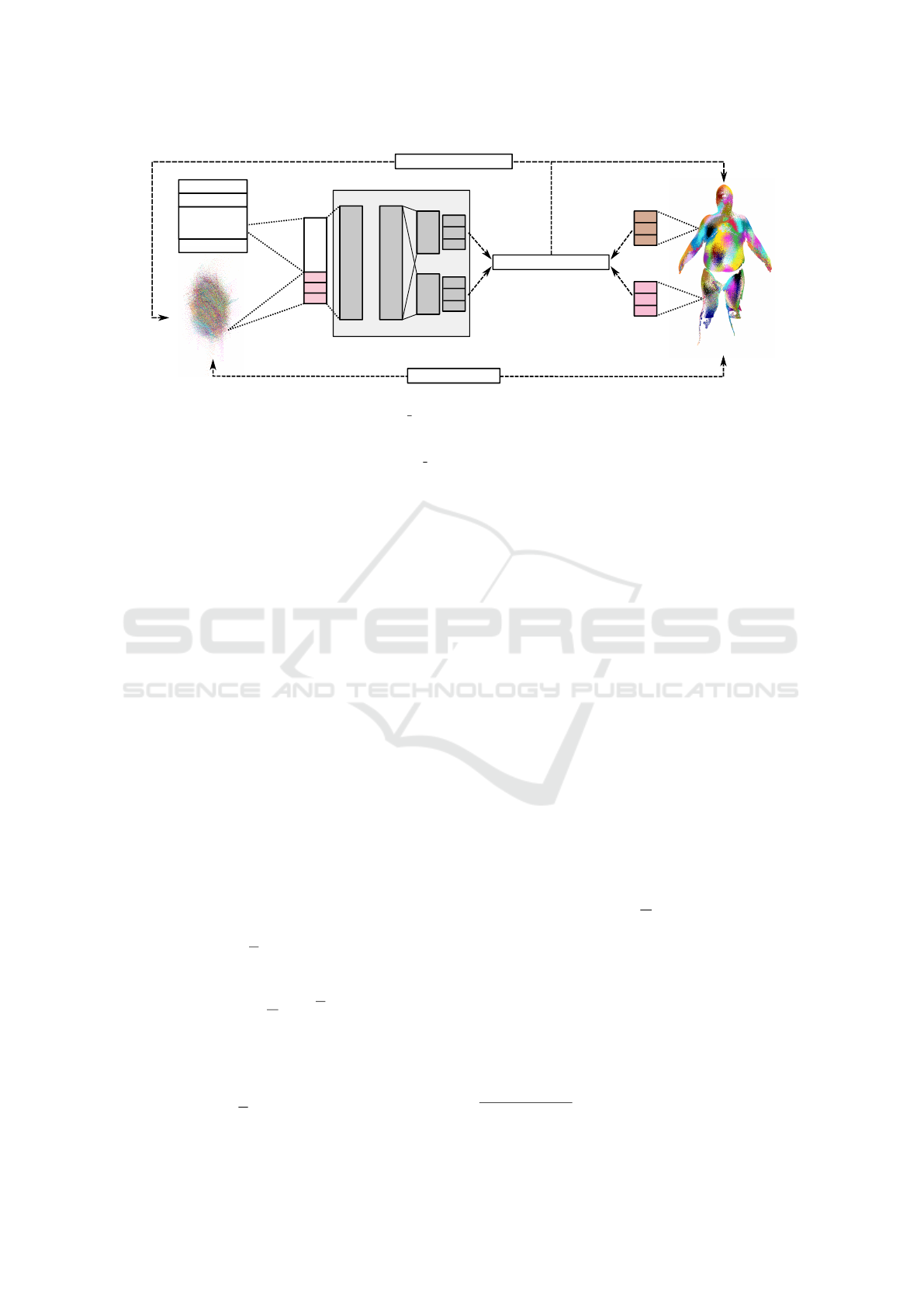
Figure 1: The topology and algorithms dedicated to NeuralQAAD. The initial assignment between the input point cloud Q

and a target point cloud P is determined by QAAD GREEDY. P is described by a latent vector l

and stored in the lookup

table L. A point q

is processed along with l

by a shared MLP to create common features. Subsequently, the common features

and q

are folded by a patch-speciﬁc MLP. The optimizer updates the input point q

, the latent code l

, and all MLP parameters

while improving the initial assignment through QAAD REASSIGNMENT.

3 METHOD

In the following, we give a formal description of the

addressed problem and derive constraints for a corre-

sponding deep learning solution. We then construct a

neural network architecture based on the concept of

folding (Yang et al., 2018) that satisﬁes these con-

straints. Finally, we demonstrate how to train this

architecture by designing and efﬁciently solving a

quadratic assignment problem. Figure 1 shows an

overview of the proposed NeuralQAAD architecture.

3.1 Problem Formulation

Given a set S = {P

| 1 ≤ i ≤ N} of 3D point clouds



i j

∈ R

| 1 ≤ j ≤ M



(1)

all having the same number of points, we seek for a

pair of functions f ,g where f : R

3·M

7→ R

,l  M en-

codes a point cloud into a lower dimensional feature

vector

= f (P

) ∈ R

, (2)

and g : R

7→ R

3·M

decodes the feature vector l

back

into a point cloud

= g(l

) (3)

such that the error

E( f ,g) =

∑

i=1

d(P

), (4)

is minimal with respect to some function d which

measures the similarity of two point clouds. As dis-

cussed in Section 2.2, folding transforms equation (3)

into

= g(l

,Q), (5)

where Q =



| 1 ≤ j ≤ M



is a single ﬁxed input

point cloud.

As point clouds possess no explicit neighborhood

information and are invariant to permutations, the en-

coder function f should also have these properties.

Therefore, we further divide f into a pointwise local

feature descriptor

f transforming the pointset P

into

a feature set



f (p

i j

) | 1 ≤ j ≤ M



(6)

and a permutation-invariant global feature descriptor

f which converts the feature set into a lower dimen-

sional feature vector

f (

) ∈ R

. (7)

Likewise, substituting the decoder function g with a

pointwise reconstruction function ˆg changes (5) into



i j

| 1 ≤ j ≤ M



with

i j

= ˆg(

). (8)

Thus, instead of ﬁnding two functions f ,g that mini-

mizes (4), our objective is now to ﬁnd three functions

f , ˆg and

f that minimize

f , ˆg,

f ) =

∑

i=1

). (9)

Minimizing (9) using deep learning algorithms, in

general, is very memory and computational intensive.

For example, a comparably small batch of 32 point

clouds each consisting of M = 65000 points is equal

to processing a rather large batch of around 2653

MNIST

images. Therefore the realization of

f , ˆg

and

f through deep neural networks requires compu-

tationally efﬁcient and memory-optimized methods as

presented in the following.

http://yann.lecun.com/exdb/mnist/

VISAPP 2022 - 17th International Conference on Computer Vision Theory and Applications

814

3.2 EM-kD

The measure d for the similarity of point clouds is

typically chosen to be either the Chamfer distance

(Groueix et al., 2018; Zhao et al., 2019)

(

P,P) =

∑

p∈P

min

p∈

p −

∑

p∈

min

p∈P

p −

(10)

or the augmented Chamfer distance (Chen et al.,

2020)

(

P,P) = max







∑

p∈P

min

p∈

p −

∑

p∈

min

p∈P

p −







(11)

with previously detected weaknesses (Liu et al., 2020;

Achlioptas et al., 2018).

Compared to the Chamfer distance, the Earth

Mover Distance (EMD)

EMD

(

P,P) = min

φ:P→

∑

p∈P

p − φ(p)

(12)

is considered to be more representative for visual vari-

eties (Liu et al., 2020; Achlioptas et al., 2018) in case

that φ is (almost) a bijection. We deﬁne

argd

EMD

(

P,P) = {(p,

p = φ(p))}

p∈P

(13)

as the linear assignment problem (LAP) imposed by

the EMD.

Since the use of the EMD even for moderately

large point clouds leads to impracticable runtimes, we

introduce a divide-and-conquer approximation of the

real EMD, which we call EM-kD. The EM-kD is de-

ﬁned as

EM−kD

(

P,P) =

∑

(

P ,P )∈k

(

P)∇k

(P)

EMD

(

P , P ), (14)

where the k

function constructs k-d tree subspaces

and ∇ deﬁnes the diagonal product that enumerates

the canonical subspace pairs. Afterwards, the (ap-

proximated) EMD between each subspace pair is

measured. In all our experiments we use the auction

algorithm as an EMD approximation.

The EM-kD closely approximates the EMD as can

be seen by considering the following two cases. First,

we assume that the low frequencies of both point

clouds are similar, i.e., the k-d subspaces will also

be similar. Here, the EM-kD may slightly overesti-

mate the EMD at most at the subspace boundaries.

The second case considers the situation where the low

frequencies of both point clouds are different and the

k-d subspaces are different as well. In this situation,

the EM-kD may signiﬁcantly overestimate the EMD.

Overall, EM-kD judges similar to the EMD, but pe-

nalizes very dissimilar point clouds even more.

As a side beneﬁt, the EM-kD may also be well

suited for other tasks where the EMD is typically

used, such as point cloud completion. While being

a reasonable upper bound of the true EMD, the EM-

kD is greatly scaleable as the subtask size of the auc-

tion algorithm can be controlled through the depth of

the k-d trees. In our experiments, using the EM-kD

reduces the runtime by more than an order of magni-

tude, more precisely by a factor of 36.

In all our experiments, we used the EM-kD to

evaluate NeuralQAAD. In Section 3.4 we present a

training procedure to implicitly optimizing the EM-

kD and hence the EMD.

3.3 Network Architecture

In the following, we discuss the three key compo-

nents that we have identiﬁed for a successful imple-

mentation of a scalable autodecoder for point clouds

based on a deep neural network. Since our approach

is mainly motivated by a Quadratic Assignment Prob-

lem and realizes an Auto Decoder, we call it Neu-

ralQAAD.

First, NeuralQAAD follows the idea of folding.

In contrast to previous work that folds a ﬁxed (Yang

et al., 2018) or trainable (Deprelle et al., 2019) point

cloud by uniformly sampling a speciﬁc manifold such

as a square, we choose to deform a random sample of

the target data set as this is very likely to be closer to

any other sample than an arbitrary primitive geome-

try and thus is better suited for initialization. For a

dataset with strong low frequency changes, clustering

of multiple random examples may be even more ad-

vantageous, but we leave this for future research as it

turned out to be not beneﬁcial in our experiments.

Second, we found that splitting the input point

cloud into K many patches that are independently

folded (Deprelle et al., 2019), i.e. K independent mul-

tilayer perceptrons (MLPs), is essential but also uses

resources highly inefﬁciently. Each patch has its own

set of parameters and thus its own set of extracted fea-

tures. Increasing the number of patches and thus the

number of MLPs, quickly limits their potential depth.

We observe that weight sharing across the ﬁrst layers

of each MLP does not decrease the performance, but

enables the realization of deeper and/or wider archi-

tectures with the same number of parameters. Sim-

ilarly, low-level feature sharing can be used to scale

the number of patches.

Third, as discussed in Section 3.1, a batch of large

point clouds may not be processed at once. To cope

with this problem, NeuralQAAD only folds a sam-

NeuralQAAD: An Efﬁcient Differentiable Framework for Compressing High Resolution Consistent Point Clouds Datasets

815

ple from each point cloud of a batch during a single

forward pass. Since the latent code

of an instance

depends on all its related points, the encoding func-

tion

f needs to be adapted. We realize

f as a trainable

lookup table and thus renounce the explicit calcula-

tion of the pointwise function

f . In addition to our

motivation for autodecoders to minimize memory us-

age, (Park et al., 2019) claims that this topology uti-

lizes computational resources more effectively.

Considering the three constituents just discussed,

the problem of ﬁnding functions

f , ˆg and

f that min-

imize (9) can now be rephrased into the problem of

training several multilayer perceptrons MLP

, one for

each input patch Q

, and a lookup table L ∈ R

N×l

such

that

E(MLP,L,Q) =

∑

i=1

d(P

), (15)

is minimized, where the elements of

are given as

i, j

= MLP

k, j

),k ∈ K. (16)

Without loss of generality, we do not explicitly state

the split into various patches to simplify notation in

the following. The inverse assignment from each pre-

dicted point to its source point is given by q

k, j

MLP

i, j

),k ∈ K.

3.4 Training

Optimizing NeuralQAAD only on subsets of the in-

put point cloud Q directly affects the construction of

the loss function. The common pattern for calculat-

ing a distance between points clouds is similar to a

registration task that can be split into the two steps

1. Identifying a suitable matching between both

point clouds.

2. Determine the actual deformation of one point

cloud to the other.

Gradient descent is only done for the second step

whereas the ﬁrst step characterizes how appropriate a

metric is. Apart from the fact that the Chamfer dis-

tance is not reliable and the EMD is not tractable,

another general consideration comes into play: The

matching that steers the folding process has to comply

with the predominant bias of neural networks, which

is smoothing. Therefore, we choose a matching that

allows the optimizer to follow the quadratic assign-

ment problem described next.

Given an input point cloud Q, a target point cloud

P, a weight function w(p,

p) =

p −

, and a ﬂow

function f (q,

q) =

/w(q,

q) we want to ﬁnd a bijective

mapping A : Q 7→ P such that

E(A) =

∑

q∈Q

f (q,

q) · w(A(q), A(

q)) (17)

is minimized. Intuitively speaking, this means that by

solving this quadratic assignment problem, we assure

that points close to each other in Q are matched with

points close to each other in P. Note that LAPs do not

exhibit this property and, hence, might inhibit gra-

dient descent. By construction, minimizing the dis-

tances between all QAP matches optimizes any cri-

terion like the EMD, EM-kD or Chamfer distances,

too.

Algorithm 1: Calculate an initial QAP solution A between a

target point cloud P and the image

P of an input point cloud

Q. The image

P is calculated by the NeuralQAAD MLP

given a latent vector l.

procedure QAAD GREEDY(l,Q,P)

// Predict input point cloud

P = MLP(l,Q)

// Set of initial QAP solution

A =

// Assignment for each canonical k-d tree subspace pair

for (

P ,P ) ∈ k

(

P)∇k

(P) do

// Matching of EMD

A = arg d

EMD

(

P ,P )

// If duplicates exist, use the smallest distance only

for (

p,p) ∈ A do

if @(

p,p) ∈ A : k(

p − p)k < k(

p − p)k then

A = A ∪ {(MLP

(l,

p),p)}

// Randomly assign the remaining points

for (

p,p) ∈ A do

if @(MLP

(l,

p),

p) ∈ A then

p ∼ uni f orm({

p ∈ P |@(q,

p) ∈ A})

A = A ∪ {(MLP

(l,

p),

p))}

// Return the initial assignment

return A

On ﬁrst sight, QAPs seem to be harder to solve

than LAPs. However, we do not need to solve them

explicitly, but remove the limitation of the optimizer

of following a linear assignment. The ﬁrst step is a

greedy algorithm called QAAD GREEDY that gen-

erates an initial matching before gradient-descent.

The second step is a dynamic reassignment algorithm

called QAAD REASSIGNMENT, that monotonically

improves equation (15). During our experiments it

became evident that neither of the two steps alone

lead to a superior solution. The novel shared Neu-

ralQAAD architecture can also be trained on the aug-

mented Chamfer Distance training procedure which

already results in a signiﬁcant performance improve-

ment and does not produce any additional assignment

overhead at all, but still is not as good as our QAAD

training scheme (see Section 4).

QAAD

GREEDY (see Algorithm 1) is conceptu-

ally similar to calculating the EM-kD. Instead of us-

ing the calculated distance between the input and the

target point cloud the determined LAP matches are

used as the initial assignment solution. To establish a

VISAPP 2022 - 17th International Conference on Computer Vision Theory and Applications

816

Algorithm 2: Reﬁning the initial QAP solution A for a

query of points Q ⊂ Q of the input point cloud Q. At

this, the image

P of the query given a latent code l is con-

structed by the current state of the NeuralQAAD MLP

and evaluated against the target point cloud P. However,

for efﬁciency only a subset P ⊂ P of the target is consid-

ered for reassignment.

procedure QAAD REASSIGNMENT(l,Q , P , A)

for q ∈ Q do

// Predict input subset and assign their nearest

// neighbors in target subset

A(q) = argmin

p∈P

MLP(l,q) − p

// Check current loss

= kMLP(l,q) − A(q)k

+kMLP(l,A

−1

(A(q))) − A(q)k

// Check loss after hypothetical reassignment

= kMLP(l,q) − A(q)k

+kMLP(l,A

−1

(A(q))) − A(q))k

// Decide where reassignment is beneﬁcial

if L

≤ L

then

// Delete old assignment

A = A \ {(q,A(q))}

A = A \ {(A

−1

(A(q)), A(q))}

// Add new assignment

A = A ∪ {(q,A(q))}

A = A ∪ {(A

−1

(A(q)), A(q))}

// Return the reﬁned assignment

return A

perfect matching, which is not guaranteed by the auc-

tion algorithm, the input point closest to a repeat-

edly chosen target point is matched. Any remain-

ing points are randomly matched. Like for the EM-

kD, QAAD GREEDY can be efﬁciently parallelized

on a GPU. Even for the largest tested dataset D-Faust

(Bogo et al., 2017) QAAD GREEDY runs only min-

utes. Additionally, since it only runs once, the runtime

is negligible considering the common training time of

neural networks.

Since the input point cloud is trainable,

QAAD GREEDY may make assignment errors

at subspace borders and the initial matching is

still an approximation of a linear assignment.

QAAD REASSIGNMENT (see Algorithm 2) con-

ducts reassignments during gradient descent that ease

the training of NeuralQAAD. At this, given a latent

code, a sample of the input point cloud is predicted

and the nearest neighbor from a sample of the target

point cloud is found for each prediction. This can

be efﬁciently done in parallel on a CPU using k-d

trees or other suitable data structures. Newer GPU

architectures that refrain from warp-based computa-

tion also allow for efﬁcient GPU implementations.

The k-d trees are build and queried with only a

few samples per training step and, hence, add little

overhead. Subsequently, the input points that are

actually assigned to the nearest neighbors are also

predicted. Reassignment is based on comparing the

summed loss of both predictions under the actual

matching with the summed loss of both predictions

after a hypothetical pointwise swap. In case the latter

loss is smaller, a reassignment is conducted. Hence,

each reassignment is guaranteed to reduce the error

deﬁned by equation (15). More importantly, the

optimizer is no longer biased towards minimizing the

distance of an optimal linear assignment.

The distance measure in this algorithm can be ar-

bitrarily chosen, but due to the targeted EM-kD, we

rely on the mean squared error. As we only process

point cloud subsets, we enforce a sampling proce-

dure that outputs the same number of points for each

patch. This allows us to efﬁciently implement Neu-

ralQAAD as a grouped convolution. In contrast to

previous implementations that sequentially run each

MLP per patch, we can make use of all GPU resources

and achieve a signiﬁcant speedup that makes using

hundreds of patches practical for the ﬁrst time.

4 EXPERIMENTS

In this section, we validate NeuralQAAD and its un-

derlying assumptions. We start with an overview of

the datasets used and some implementation details.

Subsequently, we show that NeuralQAAD performs

signiﬁcantly better on high resolution points clouds

than existing approaches. Speciﬁcally, we compare

against the AtlasNetV2 deformation architecture (De-

prelle et al., 2019), the only other state-of-the-art dif-

ferentiable approach that is out-of-the-box applica-

ble to point clouds with more than a few thousand

points. Finally, we demonstrate the beneﬁt of each

NeuralQAAD design choice in an ablation study and

the robustness of our approach in the number of sam-

pled training points.

4.1 Datasets

Our experiments are based on the three different

datasets COMA (Ranjan et al., 2018), D-Faust (Bogo

et al., 2017) and Skulls. COMA, captures 20466

scans of extreme expressions from 12 different indi-

viduals captured by a multi-camera stereo setup. D-

Faust, is a 4D full body dataset that includes 40 000

multi-camera scans of humans in motion. We use

about 6576 scans that contain more than 110000

points and about 13 744 scans that contain more than

130000 points from COMA and D-Faust respectively.

Skulls is a new artiﬁcially generated point cloud

dataset constructed using a multilinear model (Achen-

bach et al., 2018) that is based on a skull template ﬁt-

NeuralQAAD: An Efﬁcient Differentiable Framework for Compressing High Resolution Consistent Point Clouds Datasets

817

ted to 42 CT scans of human skulls (Gietzen et al.,

2019). The dataset consists of 4096 point clouds.

Each point cloud is composed of 65 536 points and

includes ﬁne-grained parts such as the nasal bones or

teeth. In contrast to the other datasets, it consists not

only of surfaces but also of volumetric structures. We

will make this dataset public as a new high resolution

point cloud test dataset.

4.2 Implementation Details

For all our experiments we implemented the Neu-

ralQAAD folding operation with six fully connected

layers with output dimensions 256-128-128-128-64-

3 using PyTorch. In this implementation, the ﬁrst

four layers are shared across all patches (see Fig-

ure 1 for an architecture overview). To guarantee the

same number of parameters for the AtlasNetV2 de-

coder while allowing it to be sufﬁciently deep, wide,

and computationally tractable we construct the fold-

ing operation of AtlasNetV2 with four layers of size

128 (no sharing) and adapt the number of patches if

needed. SELU (Klambauer et al., 2017) is applied as

a nonlinearity to every but the output layer for both

NeuralQAAD and AtlasNetV2. Adam (Kingma and

Ba, 2015) is used as the optimizer and initialized with

a learning rate of 0.001. We sample 4096 points for

COMA as well as D-Faust and 2048 points for Skulls

per instance and training step, resulting in low GPU

memory consumption.

AtlasNetV2 is trained until we can no longer ob-

serve any signiﬁcant improvement, which was the

case for all data sets after 150 epochs at the latest.

To show that our architecture is also superior with-

out our novel QAAD training scheme we also train

NeuralQAAD for 150 epochs with the AtlasNetV2

training scheme. Essentially, this means minimiz-

ing the augmented Chamfer loss on point cloud sam-

ples. For this purpose, we deploy a PointNet encoder,

too, which we discard as soon as our QAAD training

scheme is utilized. Nevertheless, the PointNet em-

beddings are reused to initialize the lookup table. For

all experiments except the convergence NeuralQAAD

experiment, we train for 450 additional epochs. All

experiments are conducted on TITAN RTX GPUs

and a AMD Ryzen™ Threadripper™ 3970X CPU.

In comparison, the experiments of AtlasNetV2 have a

noticeably longer runtime than those of NeuralQAAD

since we use the released sequential implementation

of AtlasNetV2. For instance, training AtlasNetV2 on

D-Faust takes over a day whereas NeuralQAAD only

requires two hours. For all experiments, we use the

same hyperparameters for the auction algorithm i.e.

100 iterations with an epsilon of 1. The EM-kD is

calculated with a subspace size of 1024.

4.3 Reconstruction of High Resolution

Point Clouds

Skulls: The Skulls dataset contains point clouds that

can be linearly reduced to 42 latent variables using

principal component analysis. Additionally, in our

experiments, we nonlinearly compress each skull to a

latent vector of size 10. Although this seems to be an

easy task at ﬁrst sight, results of AtlasNetV2 demon-

strate the contrary.

We process Skulls in a batch size of 16 instances

and use 16 patches for both NeuralQAAD and At-

lasNetV2. The visual results can be seen in Figure

2. NeuralQAAD is able to recover almost all low

as well as high frequencies. In contrast, AtlasNetV2

fails in both. From the side view, it can be clearly

recognized that detailed and non-manifold structures

as teeth and the nasal area are lost by AtlasNetV2

to a huge extent but can be fully reconstructed by

NeuralQAAD. In addition, rather coarse structures

like the eye socket (front view) or the skullcap (front

and side view) are badly recovered by AtlasNetV2,

whereas NeuralQAAD does not suffer. We mainly

attribute the better volumetric reconstruction capabil-

ities to the improved training procedure. However,

also the effects of weight sharing can be observed

visually. AtlasNetV2 clearly struggles in gluing to-

gether individual patches. This does not seem to be

an issue for NeuralQAAD that works on shared low

level features. The visual impressions are strongly

supported by the measured EM-kD losses stated in

Table 1. Training on the augmented Chamfer loss

alone leads to an improvement of 21% in terms of

EM-kD. After training our approach to convergence,

we even get an improvement of 78% and achieve a

compression ratio of 3311:1 (# of dataset ﬂoats : # of

network parameter and embedding ﬂoats).

D-Faust: The D-Faust dataset predominantly con-

tains low-frequency structures. We compress each

instance to a latent code of size 256. Training is

conducted with batches of size 16 while using 128

patches for NeuralQAAD. To ensure comparability in

the number of parameters AtlasNetV2 can only uti-

lize 28 patches. Visual results are depicted in Figure

3a. Unlike the volumetric Skulls dataset, here we can

recover a surface for each point cloud to facilitate vi-

sual comparison of reconstruction results. For surface

reconstruction, we used the simple ball-pivoting algo-

rithm (Bernardini et al., 1999) with identical hyperpa-

rameters for all experiments. From all perspectives, it

becomes evident that AtlasNetV2 merges even coarse

structured extremities and, as with Skulls, struggles to

VISAPP 2022 - 17th International Conference on Computer Vision Theory and Applications

818

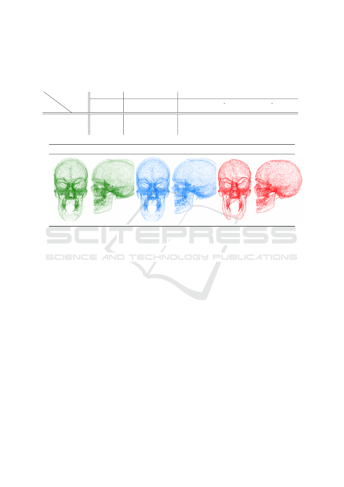
Table 1: Reconstruction EM-kD for the datasets Skull, D-Faust and COMA. Convergence is indicated with ∞. On all datasets

NeuralQAAD performances signiﬁcantly better than the previous state-of-the-art AtlasNetV2 even if trained only with the

augmented Chamfer loss. For the D-Faust dataset, NeuralQAAD achieves signiﬁcant improvements with and without QAP

training, indicating that the scalability of NeuralQAAD in the number of patches is the main performance factor. However,

for the COMA dataset both the scalability in the number of patches as well as the QAP training procedure lead to huge

performance jumps. For Skulls, mainly the novel QAP training procedure improves on the current state of the art.

Data

Architecture

Trained with

Epochs

AtlasNetV2 NeuralQAAD & Encoder NeuralQAAD

Aug. Chamfer Aug. Chamfer MSE + QAAD GREEDY + QAAD REASSIGN.

∞ (=150) 150 600 600 600 ∞

Skulls 30.681 24.004 419.230 18.312 10.481 6.708

D-Faust 0.076 0.023 0.187 0.015 0.011 0.010

COMA 200.083 139.230 2448.076 74.893 47.593 18.554

NeuralQAAD Original AtlasNetV2

Figure 2: Front and side views on NeuralQAAD reconstructions of Skulls (Achenbach et al., 2018). Each skull is compressed

to a latent vector of size 10. Low as well as high frequencies can be mostly recovered by NeuralQAAD in contrast to

AtlasNetV2 that fails on low frequencies like the skullcap or on high frequencies like the teeth.

stitch together individual patches. NeuralQAAD, by

contrast, is able to almost fully recover all prevalent

structures and forming a smooth surface across patch

borders.

The EM-kD reconstruction losses for D-Faust

stated in Tab. 1 show a signiﬁcant improvement

through NeuralQAAD. However, they tell a differ-

ent story as for Skulls. Already after training Neu-

ralQAAD with the augmented Chamfer distance, the

EM-kD decreases by about 69%. Further, our train-

ing scheme leads to a total drop in EM-kD of 86%

after convergence and achieves a compression ratio

of 1144:1. Combined, both numbers indicate that the

scalability of NeuralQAAD in the number of patches

is the dominant factor of performance for D-Faust

whereas the training scheme plays a minor role.

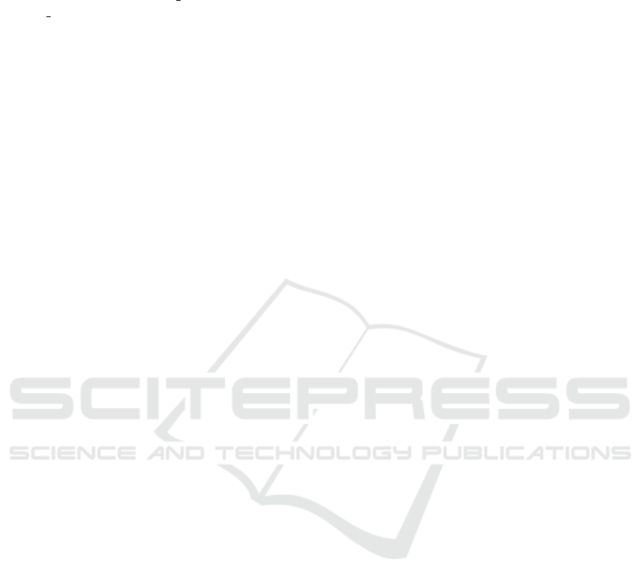
The D-Faust experiments reveal another interest-

ing observation. In Figure 4 the trainable input point

clouds are shown. Although initialized with a random

example of the respective dataset, only for D-Faust a

full deformation can be noticed. The egg-like struc-

ture seems to be favorable if strong low frequency

changes occur which is not the case for Skulls and

COMA (see next Section).

COMA: COMA is the most challenging dataset as

each point cloud contains almost as many points as

those of D-Faust but is restricted to the facial area and,

hence, captures an enormous amount of details. As

for D-Faust, we compress each instance into a latent

code of size 256, conduct training with a batch size

of 16, and make use of 128 patches for NeuralQAAD

as well as 28 patches for AtlasNetV2. Surface recon-

structions are shown in Figure 3b. For both instances

shown, NeuralQAAD is found to capture way more

ﬁne-grained structures than AtlasNetV2 while being

less noisy. Even coarse structures like the ear in the

ﬁrst instance can not be recovered by AtlasNetV2.

The EM-kD outcomes stated in Table 1 suggest

that for COMA the number of patches as well as the

QAP training scheme are essential and neither alone

sufﬁces. Training NeuralQAAD on the augmented

Chamfer distance achieves a 30% better performance

than AtlasNetV2. Applying the QAP training proce-

dure further improves NeuralQAAD by 90% overall

after convergence and results in a compression ratio

of 748:1.

NeuralQAAD: An Efﬁcient Differentiable Framework for Compressing High Resolution Consistent Point Clouds Datasets

819

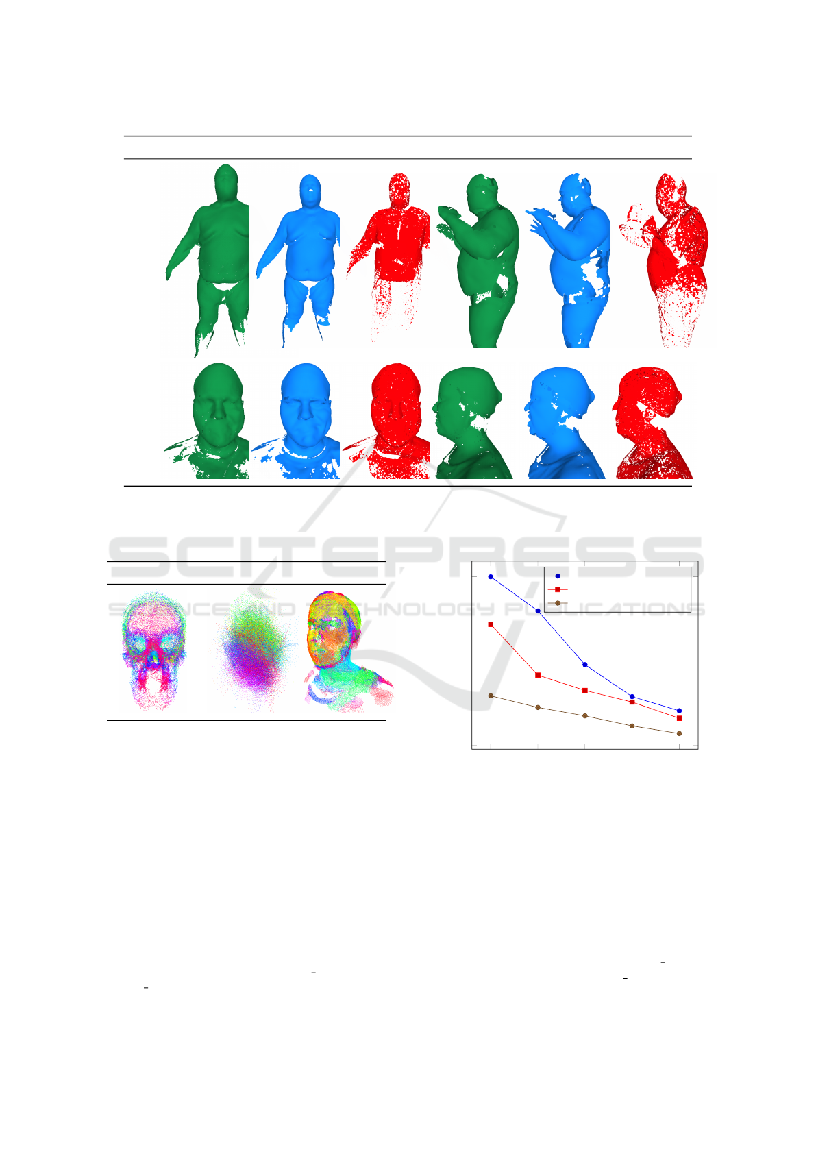
NeuralQAAD Original AtlasNetV2 NeuralQAAD Original AtlasNetV2

Figure 3: a) Front and side views on NeuralQAAD reconstructions of D-Faust (Bogo et al., 2017). The differences between

NeuralQAAD and AtlasNetV2 are clearly visible as AtlasNetV2 is not able to recover even coarse structures like extremities.

b) Front and side views on NeuralQAAD reconstructions of COMA (Ranjan et al., 2018). As for D-Faust, most detailed

structures are reconstructed by NeuralQAAD whereas AtlasNetV2 even looses coarse structures.

Skulls D-Faust COMA

Figure 4: Combined trainable input patches after QAP

training for the evaluated dataset. Colors reﬂect assignment

to patches. For Skulls and COMA, datasets mostly deﬁned

by changes in high frequencies, the input point clouds looks

like noisy instances. D-Faust, mostly deﬁned by changes

in low frequencies, exhibits a fully deformed input point

cloud.

4.4 Ablation Study & Scalability

In this section we ground the major and novel de-

sign choices made for NeuralQAAD. In the preceding

section, we already discussed the number of patches

as well as shared low-level features as the key suc-

cess factors for D-Faust and COMA proving the con-

cept of weight sharing. However, we did not dis-

cuss the isolated impact of QAAD GREEDY and

QAAD REASSIGNMENT, yet.

100

150

# Sampled Points

EM-kD

AtlasNetV2

NeuralQAAD (Only Arch.)

NeuralQAAD

Figure 5: EM-kD for AtlasNetV2, NeuralQAAD architec-

ture trained on the augmented Chamfer distance, and Neu-

ralQAAD trained with our training scheme related to the

number of sampled points per training step. The Skulls

dataset is used.

In a baseline experiment (see MSE & Decoder in

Table 1) we trained NeuralQAAD to minimize the

MSE of a random assignment. As expected, this

culminates in extraordinary bad results as the crite-

rion does not even follow the properties of a LAP.

In the subsequent experiment (see QAAD GREEDY

in Table 1), we observe that QAAD GREEDY solves

VISAPP 2022 - 17th International Conference on Computer Vision Theory and Applications

820

this issues but can clearly not be made responsi-

ble for the overall performance of NeuralQAAD.

Additionally applying QAAD REASSIGNMENT (see

QAAD REASSIGNMENT in Table 1) and, hence, fol-

lowing the smoothing bias of neural networks, boosts

the results again. In summary, the conducted experi-

ments strongly support the capabilities and the neces-

sity of the proposed contributions.

The behavior of NeuralQAAD, in the case where

the number of sampled points is reduced, is very ro-

bust. Figure 5 shows that NeuralQAAD, with and

without our training scheme, is always superior to

AtlasNetV2, regardless of the number of sampled

points. More importantly, when the number of sam-

pled points is reduced, the performance loss is signiﬁ-

cantly lower than with AtlasNetV2. The observed ro-

bustness to sampling demonstrates the efﬁciency and

scalability of NeuralQAAD with respect to the size

of the point clouds to be processed. This also equips

NeuralQAAD for the future, in which the resolution

of point clouds will most probably continue to in-

crease in most areas.

5 CONCLUSION

We introduced a new scaleable and robust point

cloud autodecoder architecture called NeuralQAAD

together with a novel training scheme. Its scalability

comes from low level feature sharing across multiple

foldable patches. In addition, refraining from classi-

cal encoders makes NeuralQAAD robust to sampling.

Our novel training scheme is based on two newly

developed algorithms to efﬁciently determine an ap-

proximate solution that follows the smoothing bias of

neural networks. We showed that NeuralQAAD pro-

vides better results than the previous state-of-the-art

applicable to high resolution point clouds. Our com-

parisons are based on the EM-kD, a novel scalable

and fast upper bound for the EMD. In our experi-

ments, the EM-kD has proven to reasonably reﬂect

visual differences between point clouds.

The next steps will be to make our approach ap-

plicable to generative models and to bridge the gap

to correspondence problems. Although at ﬁrst glance

generative tasks seem to be a straightforward ex-

tension, preliminary results have shown an unstable

training process. Recent advancements in continuous

learning might be adaptable to diminish the effects of

sampling.

REFERENCES

Achenbach, J., Brylka, R., Gietzen, T., zum Hebel, K.,

Sch

omer, E., Schulze, R., Botsch, M., and Schwa-

necke, U. (2018). A multilinear model for bidirec-

tional craniofacial reconstruction. In VCBM 2018,

pages 67–76.

Achlioptas, P., Diamanti, O., Mitliagkas, I., and Guibas,

L. J. (2018). Learning representations and generative

models for 3d point clouds. In ICML 2018, pages 40–

49.

Beckman, M. and Koopmans, T. (1957). Assignment prob-

lems and the location of economic activities. Econo-

metrica, pages 53–76.

Bernardini, F., Mittleman, J., Rushmeier, H. E., Silva, C. T.,

and Taubin, G. (1999). The ball-pivoting algorithm

for surface reconstruction. IEEE Trans. Vis. Comput.

Graph., (4):349–359.

Bertsekas, D. P. (1988). The auction algorithm: A dis-

tributed relaxation method for the assignment prob-

lem. Ann. Oper. Res., (1–4):105–123.

Bogo, F., Romero, J., Pons-Moll, G., and Black, M. J.

(2017). Dynamic FAUST: registering human bodies

in motion. In CVPR 2017, pages 5573–5582.

Bruna, J., Zaremba, W., Szlam, A., and LeCun, Y. (2014).

Spectral networks and locally connected networks on

graphs. In ICLR 2014.

Burkard, R. E. (1984). Quadratic assignment problems.

European Journal of Operational Research, (3):283–

289.

Chen, S., Duan, C., Yang, Y., Li, D., Feng, C., and Tian, D.

(2020). Deep unsupervised learning of 3d point clouds

via graph topology inference and ﬁltering. IEEE

Trans. Image Processing, 29:3183–3198.

Deprelle, T., Groueix, T., Fisher, M., Kim, V. G., Russell,

B. C., and Aubry, M. (2019). Learning elementary

structures for 3d shape generation and matching. In

NIPS 2019, pages 7433–7443.

Edmonds, J. and Karp, R. M. (1972). Theoretical improve-

ments in algorithmic efﬁciency for network ﬂow prob-

lems. J. ACM, (2):248–264.

Fan, H., Su, H., and Guibas, L. J. (2017). A point set gen-

eration network for 3d object reconstruction from a

single image. In CVPR 2017, pages 2463–2471.

Feydy, J., S

ejourn

e, T., Vialard, F.-X., Amari, S.-i., Trouv

A., and Peyr

e, G. (2019). Interpolating between op-

timal transport and mmd using sinkhorn divergences.

In The 22nd International Conference on Artiﬁcial In-

telligence and Statistics, pages 2681–2690.

Gietzen, T., Brylka, R., Achenbach, J., zum Hebel, K.,

Sch

omer, E., Botsch, M., Schwanecke, U., and

Schulze, R. (2019). A method for automatic foren-

sic facial reconstruction based on dense statistics of

soft tissue thickness. PLOS ONE, pages 1–19.

Girdhar, R., Fouhey, D. F., Rodriguez, M., and Gupta, A.

(2016). Learning a predictable and generative vector

representation for objects. In ECCV 2016, pages 484–

499.

NeuralQAAD: An Efﬁcient Differentiable Framework for Compressing High Resolution Consistent Point Clouds Datasets

821

Goodfellow, I., Pouget-Abadie, J., Mirza, M., Xu, B.,

Warde-Farley, D., Ozair, S., Courville, A., and Ben-

gio, Y. (2014). Generative adversarial nets. In

Advances in neural information processing systems,

pages 2672–2680.

Groueix, T., Fisher, M., Kim, V. G., Russell, B., and Aubry,

M. (2018). AtlasNet: A Papier-M

ach

e Approach to

Learning 3D Surface Generation. In CVPR 2018.

Jonker, R. and Volgenant, T. (1986). Improving the

hungarian assignment algorithm. Oper. Res. Lett.,

(4):171–175.

Kingma, D. P. and Ba, J. (2015). Adam: A method for

stochastic optimization. In ICLR 2015.

Kingma, D. P. and Welling, M. (2014). Auto-encoding vari-

ational bayes. In ICLR 2014.

Klambauer, G., Unterthiner, T., Mayr, A., and Hochreiter,

S. (2017). Self-normalizing neural networks. In NIPS

2017, pages 971–980.

Kuhn, H. W. (1955). The Hungarian Method for the Assign-

ment Problem. Naval Research Logistics Quarterly,

(1–2):83–97.

Liu, M., Sheng, L., Yang, S., Shao, J., and Hu, S. (2020).

Morphing and sampling network for dense point cloud

completion. In EAAI 2020, pages 11596–11603.

Maturana, D. and Scherer, S. A. (2015). Voxnet: A 3d con-

volutional neural network for real-time object recog-

nition. In IROS 2015, pages 922–928.

Mescheder, L., Oechsle, M., Niemeyer, M., Nowozin, S.,

and Geiger, A. (2019). Occupancy networks: Learn-

ing 3d reconstruction in function space. In CVPR,

pages 4460–4470.

Park, J. J., Florence, P., Straub, J., Newcombe, R. A., and

Lovegrove, S. (2019). Deepsdf: Learning continu-

ous signed distance functions for shape representa-

tion. CoRR.

Qi, C. R., Su, H., Mo, K., and Guibas, L. J. (2017a). Point-

net: Deep learning on point sets for 3d classiﬁcation

and segmentation. In CVPR 2017, pages 77–85.

Qi, C. R., Yi, L., Su, H., and Guibas, L. J. (2017b). Point-

net++: Deep hierarchical feature learning on point sets

in a metric space. In NIPS 2017, pages 5099–5108.

Ranjan, A., Bolkart, T., Sanyal, S., and Black, M. J. (2018).

Generating 3D faces using convolutional mesh au-

toencoders. In ECCV 2018, pages 725–741.

Roveri, R., Rahmann, L.,

Oztireli, C., and Gross, M. H.

(2018). A network architecture for point cloud clas-

siﬁcation via automatic depth images generation. In

CVPR 2018, pages 4176–4184.

Sabour, S., Frosst, N., and Hinton, G. E. (2017). Dynamic

routing between capsules. In NIPS 2017, pages 3856–

3866.

Sharma, A., Grau, O., and Fritz, M. (2016). Vconv-dae:

Deep volumetric shape learning without object labels.

In ECCV 2016 Workshops, pages 236–250.

Su, H., Maji, S., Kalogerakis, E., and Learned-Miller, E. G.

(2015). Multi-view convolutional neural networks for

3d shape recognition. In ICCV 2015, pages 945–953.

Tatarchenko, M., Park, J., Koltun, V., and Zhou, Q. (2018).

Tangent convolutions for dense prediction in 3d. In

CVPR 2018, pages 3887–3896.

Wang, P., Sun, C., Liu, Y., and Tong, X. (2018). Adap-

tive O-CNN: a patch-based deep representation of 3d

shapes. ACM Trans. Graph., 37(6):217:1–217:11.

Wu, J., Zhang, C., Xue, T., Freeman, B., and Tenenbaum,

J. (2016). Learning a probabilistic latent space of ob-

ject shapes via 3d generative-adversarial modeling. In

NIPS 2016, pages 82–90.

Xu, Y., Fan, T., Xu, M., Zeng, L., and Qiao, Y. (2018).

Spidercnn: Deep learning on point sets with param-

eterized convolutional ﬁlters. In ECCV 2018, pages

90–105.

Yang, Y., Feng, C., Shen, Y., and Tian, D. (2018). Fold-

ingnet: Point cloud auto-encoder via deep grid defor-

mation. In CVPR 2018, pages 206–215.

Zadeh, A., Lim, Y.-C., Liang, P. P., and Morency, L.-

P. (2019). Variational auto-decoder: Neural gen-

erative modeling from partial data. arXiv preprint

arXiv:1903.00840.

Zhao, Y., Birdal, T., Deng, H., and Tombari, F. (2019). 3d

point capsule networks. In CVPR 2019, pages 1009–

1018.

Zhou, Y. and Tuzel, O. (2018). Voxelnet: End-to-end learn-

ing for point cloud based 3d object detection. In CVPR

2018, pages 4490–4499.

VISAPP 2022 - 17th International Conference on Computer Vision Theory and Applications

822