
RVPLAN: Runtime Verification of Assumptions in Automated Planning
Angelo Ferrando
1 a
and Rafael C. Cardoso
2 b
1
University of Genova, Genova 16145, Italy
2
The University of Manchester, Manchester M13 9PL, U.K.
Keywords:
Automated Planning, Runtime Verification, Failure Detection, STRIPS.
Abstract:
Automated planners use a model of the system and apply state transition functions to find a sequence of actions
(a plan) that successfully solves a (set of) goal(s). The model used during planning can be imprecise, either
due to a mistake at design time or because the environment is dynamic and changed before or during the plan
execution. In this paper we use runtime monitors to verify the assumptions of plans at runtime in order to
effectively detect plan failures. This paper offers three main contributions: (a) two methods (instantiated and
parameterised) to automatically synthesise runtime monitors by translating planning models (STRIPS-like) to
temporal logics (Past LTL or Past FO-LTL); (b) an approach to use the resulting runtime monitors to detect
failures in the plan; and (c) the RVPLAN tool, which implements (a) and (b). We illustrate the use of our
work with a remote inspection running example as well as quantitative results comparing the performance
of the proposed monitor generation methods in terms of property synthesis, monitor synthesis, and runtime
verification.
1 INTRODUCTION
Automated planning techniques (Nau et al., 2004) use
models of the system to search the state-space for a se-
quence of actions that can achieve the goals of the ap-
plication. Existing planners have been developed over
many years and as a result are very efficient in solv-
ing task planning problems, both in terms of speed
as well as quality/length of the resulting plan. How-
ever, complex real-world applications can be difficult
to model, above all in cyber-physical systems where
the environment is dynamic and the information may
be incomplete. In these systems, plans can fail due
to the use of outdated information or incorrect model
abstraction. When this happens, it is crucial for the
system to be able to detect plan failure, as well as trig-
gering a replanning (Fox et al., 2006) mechanism us-
ing up-to-date information. In this paper, we focus on
failure detection, but we plan to extend our approach
in future work to integrate with a replanning mecha-
nism (we expand this notion at the end of the paper).
The literature overview on verification and vali-
dation of planning and scheduling systems presented
in (Bensalem et al., 2014) categorises the verification
and validation of plan executions into runtime verifi-
a
https://orcid.org/0000-0002-8711-4670
b
https://orcid.org/0000-0001-6666-6954
cation and runtime enforcement. We argue that our
approach covers the former, while the latter is related
to the use of runtime monitors to aid in replanning and
plan repair. There are other formal methods that are
better at verifying other areas in planning, such as ver-
ification of the models used, verification of the plans
(not plan executions), verification of the planners, etc.
Runtime Verification (RV) is a lightweight formal
verification technique that checks traces of events pro-
duced by the system execution against formal proper-
ties (Bartocci et al., 2018). RV can be performed at
runtime, which opens up the possibility to act when-
ever incorrect behaviour of a software system is de-
tected. One of the most common ways to achieve
RV is through monitoring. A monitor can be seen
as a device that reads a finite trace and yields a cer-
tain verdict. It is generally less expensive than other
verification techniques, such as model checkers and
Satisfiability Modulo Theories (SMT) solvers, since
it does not exhaustively analyse all the possible sys-
tem’s executions, but only the execution trace.
RV is suitable in scenarios where there is no ac-
cess to the system under analysis (black-box), since
it only requires to analyse the traces produced by
the system execution; it does not require a model of
the system nor knowledge about its implementation.
It also finds applications in safety-critical scenarios,
Ferrando, A. and Cardoso, R.
RVPLAN: Runtime Verification of Assumptions in Automated Planning.
DOI: 10.5220/0010776500003116
In Proceedings of the 14th International Conference on Agents and Artificial Intelligence (ICAART 2022) - Volume 2, pages 67-77
ISBN: 978-989-758-547-0; ISSN: 2184-433X
Copyright
c
2022 by SCITEPRESS – Science and Technology Publications, Lda. All rights reserved
67

where a runtime failure can be extremely costly. The
presence of monitors in such scenarios helps to iden-
tify when something goes wrong (possibly reduc-
ing/avoiding unwanted side effects).
Since RV can be applied while the system is run-
ning, it can be used alongside automated planning to
deal with some of the drawbacks of using planning
solutions at runtime. If the model of the world used
by a planner is imprecise, or the system is dynamic
and continuously changes, the system needs to be able
to detect plan failure. If the system changes dynam-
ically, the resulting reality gap between the system
and the planner abstraction may cause unexpected be-
haviours. For instance, an action that was rightfully
selected to be executed as part of a plan might fail
at runtime due to violations of its preconditions, or
it might produce unexpected results. Moreover, usu-
ally systems are dynamic, and to use a planner in a
safe and sound way, we need to recognise when the
assumptions made by the planner are no longer met
by the system. Checking the assumptions of a plan at
runtime is often dealt with ad-hoc methods that have
to be specifically designed and implemented for each
action. Runtime monitors allows us to perform this
failure detection at runtime using formal verification,
and in this paper we show how these monitors can be
automatically generated from the planning specifica-
tion, making the process of checking the assumptions
completely domain-independent.
In this paper we introduce an approach for fail-
ure detection that uses monitors to verify at runtime
the assumptions of the actions that are generated by
a classical planner. In particular, we show how to
automatically synthesise runtime monitors with two
different methods: (a) the instantiated action moni-
toring uses the actions of a plan that was generated
as a solution to a planning problem, as well as the
actions descriptions; or (b) the parameterised action
monitoring uses only the actions descriptions. Then,
we describe how these monitors can be used to de-
tect violations in the assumptions of a plan at run-
time. Finally, we discuss the implementation details
of our RVPLAN tool and present results of exper-
iments comparing the performance of both methods
(instantiated and parameterised) in terms of property
synthesis (translation time), monitor synthesis (creat-
ing the monitor), and runtime verification (the time it
takes to verify the properties).
The rest of the paper is organised as follows. Sec-
tion 2 contains the related work in automated plan-
ning, in particular approaches that deal with plan fail-
ure detection. In Section 3 we discuss the necessary
background on automated planning and show a run-
ning example that we use to exemplify the concepts
pertaining to our approach. We introduce our tool,
RVPLAN, in Section 4, with the instantiated action
monitoring method in Section 4.1, the parameterised
action monitoring method in Section 4.2, and our gen-
eral approach to fault detection in Section 4.3. To
evaluate our framework we present the implementa-
tion details of our tool as well as some experiments to
measure its performance in Section 5. We conclude
the paper with our final remarks and discuss future
work in Section 6.
2 RELATED WORK
ROSPlan
1
(Cashmore et al., 2015) embeds classical
task planning in the Robot Operating System (ROS)
through the addition of some ROS nodes for plan-
ning. One such node is a knowledge base that is
updated with current information related to planning
predicates through the use of manually written filters.
Actions that are dispatched to be executed are tested
before execution to make sure they are still valid (i.e.,
failure detection).
PlanSys2
2
(Mart
´
ın et al., 2021) is an alternative
to ROSPlan for performing task planning in ROS (in
particular ROS2). The novel contributions of Plan-
Sys2 include translating plans into behaviour trees
(mathematical model of plan execution), and then
auctioning the actions in these plans to components
in the system that are capable of executing them.
The main differences between ROSPlan and Plan-
Sys2 to RVPLAN are that our approach is not limited
to ROS and our monitors are automatically synthe-
sised, requiring no input from the developer.
In this paper we focus on the use of of-
fline planners, but there are many approaches that
deal with planning in an online setting. Several
approaches have integrated Belief-Desire-Intention
(BDI) agents with planning (Sardina and Padgham,
2011; Meneguzzi and Luck, 2013; Cardoso and Bor-
dini, 2019). Even though all of them support failure
detection of plans through the use of BDI agents, they
add more computation overhead than simply adding
a monitor. Furthermore, some of the translations be-
tween agents and planners are not fully automated.
In (Bozzano et al., 2011), the authors propose an
approach to on-board autonomy relying on model-
based reasoning. They discuss planning under envi-
ronment assumptions and an execution and monitor-
ing framework. Such a framework is integrated within
a generic three layers hybrid autonomy architecture,
1
https://github.com/KCL-Planning/ROSPlan
2
https://github.com/IntelligentRoboticsLabs/
ros2 planning system
ICAART 2022 - 14th International Conference on Agents and Artificial Intelligence
68

the Autonomous Reasoning Engine (ARE). The as-
sumptions are controlled at runtime, if the anomaly is
due to a change in the environment or in the expected
use of resources, then new assumptions can be com-
puted, and the rest of the plan can be validated w.r.t.
the new assumptions. If the validation succeeds then
its execution can be continued. Otherwise, replanning
with the new assumptions can be triggered.
The LAAS architecture for space autonomy appli-
cations is described in (Ghallab et al., 2001). Given
the targeted domain, the paper highlights two main
components of the architecture, failure detection/han-
dling and planning. The decision level of their archi-
tecture is particularly relevant here, as it is responsi-
ble for supervising the execution of plans. The fault
protection is done through a rule-based system that is
compiled into an automaton for execution. Execution
failure is separate to fault protection and leads to lo-
cal replanning. It is not clear how failures are detected
in their architecture, which is one of the main advan-
tages of our approach (completely automated based
on the planning specifications).
In (Mayer and Orlandini, 2015), robust plan exe-
cution is presented through plans with flexible time-
lines. Such flexible plans are translated into a net-
work of Timed Game Automata, which is then veri-
fied. Specifically, they verify whether a dynamic exe-
cution strategy can be generated by solving a reacha-
bility game. Differently from our work, their verifier
is used to guide the plan selection, while our contri-
bution is mainly focused on recognising assumption
violation. Their framework is also domain indepen-
dent, but it is less general than ours because their plan
representation must comply with the framework pro-
posed in (Mayer et al., 2016). RVPLAN is based upon
the PDDL standard (widely supported in automated
planning).
Some challenges in changing the models or ab-
stractions used in planning when the execution either
fails or produces unexpected outcomes are presented
in (Frank, 2015). The author compares these chal-
lenges to the concept of computational reflection and
shows how to relate planning models to execution
abstractions in a case study of a spacecraft attitude
planning. No implementation artifact is available and
the discussion is limited to describing potential solu-
tions. However, the discussion about abstractions and
refinements can be useful for our future work about
making changes in the actions from planning models.
None of these works exploit Runtime Verification
to validate the planner’s assumption at execution time.
Indeed, the violation detection, when present, is ob-
tained by manually implementing (hard-coding) such
a feature. Instead, in our work, we present fault detec-
tion of plans through runtime monitors that are auto-
matically generated based on the plans’ assumptions.
3 AUTOMATED PLANNING
RUNNING EXAMPLE
In this paper we consider STRIPS (STanford Re-
search Institute Problem Solver) planning (Fikes and
Nilsson, 1971). Note that even though we focus on
STRIPS-like syntax as a proof of concept for our eval-
uation experiments, our results are general and can
be ported to any planner that supports STRIPS plan-
ning. The classical planning problem, also called a
STRIPS problem, consists of a set of actions A, a
set of propositions S
0
called an initial state, and dis-
joint sets of goal propositions G
+
and G
−
describ-
ing the propositions required to be true and false (re-
spectively) in the goal state. A solution to the plan-
ning problem is a sequence of actions a
1
, a
2
, . . . , a
n
such that S = γ(...γ(γ(S
0
, a
1
), a
2
), ..., a
n
) and (G
+
⊆
S) ∧ (G
−
∩ S =
/
0). With γ(S
0
, a
1
) representing the
state transition function of applying action a
1
to state
S
0
. A sequence of actions is called a plan.
Formally, let P be a set of all propositions mod-
elling properties of world states. Then a state S ⊆ P
is a set of propositions that are true in that state. Each
action functor a (i.e., planning operator) is described
by four sets of propositions (α
+
a
, α
−
a
, β
+
a
, β
−
a
), where
α
+
a
, α
−
a
, β
+
a
, β
−
a
⊆ P. Sets α
+
a
and α
−
a
describe dis-
joint positive and negative preconditions of action a,
that is, propositions that must be true and false right
before the action a. Action a is applicable to state S
iff (α
+
a
⊆ S) ∧ (α
−
a
∩ S =
/
0). Sets β
+
a
and β
−
a
describe
disjoint positive and negative effects of action a, that
is, propositions that will become true and false in the
state right after executing the action a. If an action
a is applicable to state S then the state right after the
action a will be γ(S, a) = (S \ β
−
a
) ∪ β
+
a
. If an action a
is not applicable to state S then γ(S, a) is undefined.
A classical planner is a tuple hP, O, S
0
, Gi, with
P a set of propositions that model states (the pred-
icates), O a set of planning operators (actions)
ha, α
+
a
, α
−
a
, β
+
a
, β
−
a
i ∈ O, S
0
the set of propositions
which are initially true, and G the set of goals to
achieve.
Classical planners take as input domain (contain-
ing planning operators O) and problem (containing
initial state S
0
and goals G) files and output a plan.
In our example we have used the standard formal-
ism for classical planning PDDL (Planning Domain
Definition Language) (Mcdermott et al., 1998) which
supports STRIPS-like planning. To simplify the rep-
resentation of the problem we use the typing require-
RVPLAN: Runtime Verification of Assumptions in Automated Planning
69

ment of PDDL, which allows us to assign types to
the parameters of predicates. It is straightforward
to translate between planning representations with or
without typing. The use of typing does not have any
influence in our runtime verification approach and is
only used to improve readability of the models.
We introduce a planning scenario to motivate our
work, and we also use it to exemplify our approach in
a later section. In this example, a rover traverses a 2D
grid map to perform the remote inspection of tanks
containing radioactive material, while trying to avoid
cells with high-level of radiation. The domain file is
shown in Listing 1. The planning objects in this sce-
nario are robots, grid cells, and radiation tanks. The
following list of predicates is used: robot-at(r,x) and
tank-at(t,x) indicate the position of a robot or a tank
in a cell; up(x,y), down(x,y), left(x,y), and right(x,y)
indicate possible movements from cell x to cell y;
empty(x) is used to mark that cell x is empty; radi-
ation(x) denotes that cell x has high radiation; and in-
spected(t) represents when a tank has been inspected.
1 ( d e f i n e ( domain r e m ot e − i n s p e c t i o n )
2 ( : r e q u i r e m e n t s : t y p i n g )
3 ( : t y p e s r o b o t c e l l t a n k − o b j e c t )
4 ( : p r e d i c a t e s
5 ( r o b o t− a t ? r − r o b o t ? x − c e l l )
6 ( t a n k −a t ? t − t a n k ? x − c e l l )
7 ( up ? x − c e l l ? y − c e l l )
8 ( down ? x − c e l l ? y − c e l l )
9 ( r i g h t ? x − c e l l ? y − c e l l )
10 ( l e f t ?x − c e l l ? y − c e l l )
11 ( empt y ? x − c e l l )
12 ( r a d i a t i o n ?x − c e l l )
13 ( i n s p e c t e d ? t − t a n k ) )
14 ( : a c t i o n r i g h t
15 : p a r a m e t e r s (? r − r o b o t ? x − c e l l ? y − c e l l )
16 : p r e c o n d i t i o n ( and ( r o b o t− a t ? r ? x ) ( r i g h t
? x ?y ) ( empty ? y ) ( n o t ( r a d i a t i o n ? y ) ) )
17 : e f f e c t ( an d ( r o bo t − a t ? r ? y ) ( no t ( r o bo t − a t
? r ? x ) ) ( empty ?x ) ( n o t ( em pty ?y ) ) ) )
18 ( : a c t i o n i n s p e c t − r i g h t
19 : p a r a m e t e r s (? r − r o b o t ? x − c e l l ? y − c e l l
? t − t a n k )
20 : p r e c o n d i t i o n ( and ( r o b o t− a t ? r ? x ) ( ta n k − a t
? t ? y ) ( r i g h t ? x ? y ) ( n o t ( i n s p e c t e d ? t
) ) )
21 : e f f e c t ( an d ( i n s p e c t e d ? t ) ) )
22 )
Listing 1: Domain file for the running example.
The domain contains actions for movement in the
grid and for inspecting tanks. Movement is separated
into four actions, move up, down, left, and right. The
parameters for the movement actions are the robot
performing the action, the current cell x, and the des-
tination cell y. The preconditions include that the
robot is currently at cell x, there is a path between
rover
T
1
T
2
Figure 1: Initial state in a 3x3 grid; rover is the robot, T
1
and T
2
are the tanks to be inspected, and the green drop is
radiation.
x and y (predicate up, down, left, right depending on
the action), y is empty, and there is no radiation in y.
The effects are that the robot is no longer at x but it
is now at y, cell x is empty, and cell y is no longer
empty. Similarly, there are four actions for inspect-
ing a tank, inspect-up, inspect-down, inspect-left, and
inspect-right. Parameters are the robot, the tank, the
cell that the robot is at x, and the cell that the tank is
at y. Preconditions are that the robot is currently at x,
the tank is at y, there is a path between x and y, and
the tank has not been inspected yet. The effect is that
the tank has now been inspected. To improve read-
ability we only show the actions to move right and to
inspect-right, but the others are almost identical.
Listing 2 contains the problem description, with
the initial state illustrated in Figure 1. The first cell
in the grid is cell 0-0 (top left, first number is x axis,
second is y axis) and the last is cell 2-2 (bottom right).
Predicates that are followed by . . . indicate that these
continue to permutate using the remaining cell objects
where appropriate. An example of a plan returned by
a classical planner is shown in Listing 3.
1 ( d e f i n e ( pr o ble m p01 )
2 ( : d om a in r e m o t e − i n s p e c t i on )
3 ( : o b j e c t s c e l l 0 −0 c e l l 1 − 0 ce l l 2 − 0
4 c e l l 0 −1 c e l l 1 − 1 c e l l 2 −1
5 c e l l 0 −2 c e ll 1 − 2 c e l l 2 − 2 − c e l l
6 t a n k1 t a nk 2 − t a n k
7 r o v e r − r o b o t )
8 ( : i n i t
9 ( r o b o t− a t r o v e r c e l l 0 −0 )
10 ( t a n k −a t t a n k1 c e l l 2 −0 )
11 ( t a n k −a t t a n k2 c e l l 2 −2 )
12 ( empty c el l 1 −0 ) . . .
13 ( up c e ll 0 − 1 c e l l 0 − 0 ) . . .
14 ( down c e l l 0 −0 c e l l 0 − 1 ) . . .
15 ( r i g h t c e l l 0 − 0 c e l l 1 −0 ) . . .
16 ( l e f t c e l l 1 − 0 c e ll 0 − 0 ) . . .
17 ( r a d i a t i o n c e ll 2 − 1 ) )
18 ( : g o a l ( and ( i n s p e c t e d t an k1 ) ( i n s p e c t e d
t an k2 ) ) )
19 )
Listing 2: Problem file for the running example.
ICAART 2022 - 14th International Conference on Agents and Artificial Intelligence
70

1 ( r i g h t r o v e r c e l l 0 −0 c e ll 1 − 0 )
2 ( i n s p e c t − r i g h t r o v e r c e l l 1 − 0 c e ll 2 − 0 t an k 1 )
3 ( down r o v e r c e l l 1 − 0 c e l l 1 − 1 )
4 ( down r o v e r c e l l 1 − 1 c e l l 1 − 2 )
5 ( i n s p e c t − r i g h t r o v e r c e l l 1 − 2 c e ll 2 − 2 t an k 2 )
Listing 3: Example of solution found by a planner.
Even though initial sources of radiation can be re-
ported at planning time, at runtime the radiation levels
can change. A mechanism for detecting these changes
is necessary to ensure the safety of the robot and the
correctness of the plan.
4 RVPLAN
In this section, we show how to map the planner’s as-
sumptions into a runtime monitor and the theory be-
hind our tool. This monitor can then be used to verify
at runtime whether the system satisfies these assump-
tions. If the system behaves differently from what as-
sumed by the planner, the monitor reports a violation.
RVPLAN is meant to automate the translation
from planner’s assumptions to runtime monitors. We
present two possible methods for automatically syn-
thesising these monitors. The first uses a plan and the
set of planning operators to generate a monitor (in-
stantiated method), while the second uses only the set
of planning operators (parameterised method). Then,
we discuss how monitors generated in such a way can
be used for fault detection.
4.1 Instantiated Action Monitoring
The standard formalism to specify formal properties
in RV is propositional Linear-time Temporal Logic
(LTL) (Pnueli, 1977). Given a propositional LTL
property, a monitor can be synthesised as a Finite
State Machine (FSM) (Andreas Bauer, 2011). Given
a trace where each element is a proposition, the FSM
returns the verdict > or ⊥, if the trace satisfies (resp.
violates) the LTL property
3
. LTL, however, has only
future modalities, while it is widely recognised that
its extension with past operators (Kamp, 1968) al-
lows writing specifications which are easier, shorter
and more intuitive (Lichtenstein et al., 1985).
The definition of linear temporal logic restricted
to past time operators (Past LTL for short) is as fol-
lows (Manna and Pnueli, 1989):
ϕ = true | f alse | a | p
+
| p
−
| (ϕ ∧ϕ
0
) |
3
Additional verdicts can be used, but, since we check
safety properties, we only care about ⊥ to identify viola-
tions. For further readings (Bauer et al., 2010).
(ϕ ∨ ϕ
0
) | ¬ϕ | (ϕ S ϕ
0
) | ϕ
where a is an action, p
+
is a positive proposition,
p
−
is a negative proposition (both ground without
variables), ϕ is a formula, S stands for since, and
stands for previous-time. We also write (ϕ → ϕ
0
)
instead of (¬ϕ ∨ ϕ
0
), and Hϕ (history ϕ) instead of
¬(true S ¬ϕ). Using this logic, we can describe run-
time constraints on the preconditions of the planner’s
actions. Note that we assume the events generated by
the system execution to consist in both positive and
negative propositions. Which means, for each propo-
sition p, we have the corresponding observable events
p
+
and p
−
, which represent the event of observing the
proposition p to be true or false, respectively.
For instance, considering our running example,
we might have the proposition empty(cell 0-0)
+
,
which denotes that cell 0-0 is empty, or
empty(cell 0-0)
−
, which denotes that cell 0-0 is
not empty. Note that, p
−
and ¬(p
+
) have different
meanings (resp. p
+
and ¬(p
−
)). When we use p
−
(resp. p
+
), we denote the event corresponding to
observing proposition p being false (resp. true).
While when we use ¬(p
+
) (resp. ¬(p
−
)), we mean
any observable event which is not p
+
(resp. p
−
).
For example, empty(cell 0-0)
−
means we observe
the empty(cell 0-0) proposition to be false (i.e., the
cell is not empty). While ¬empty(cell 0-0)
+
means
we observe anything but empty(cell 0-0)
+
(i.e.,
any event is allowed apart from empty(cell 0-0)
+
),
differently from empty(cell 0-0)
−
where we must
observe empty(cell 0-0)
−
.
Given a Plan = [a
1
, a
2
, . . . , a
n
], for each action
a
i
we extract the set of preconditions instantiated
with a
i
values; namely, we get the domain action
ha
i
, α
+
a
i
, α
−
a
i
, β
+
a
i
, β
−
a
i
i ∈ O, in which we substitute all
variables according to the instantiated propositions in
a
i
. Considering the running example, the first action
in the plan was right(rover, cell
0-0, cell 1-0).
Thus, we need to check at runtime that every time
the action right(rover, cell 0-0, cell 1-0) is performed,
its preconditions are met. This can be represented as
the Past LTL formula (with rover, cell 0-0, cell 1-0
abbreviated in r, c0 and c1):
ϕ = H(right(r, c0, c1) → ((¬robot at(r, c0)
−
S
robot at(r, c0)
+
) ∧ (¬empty(c1)
−
S empty(c1)
+
) ∧
(¬right(c0, c1)
−
S right(c0, c1)
+
) ∧ (¬radiation(c1)
+
S
radiation(c1)
−
)))
which says that every time (H) we observe the
right(r, c0, c1) action, in the previous time step ()
its preconditions are met. This is obtained by check-
ing that in the past robot
at(r, c0)
+
has been observed,
and since then (S) its negation robot at(r, c0)
−
has not
been observed (the same for the other preconditions).
Intuitively, we are saying that we observed the robot
RVPLAN: Runtime Verification of Assumptions in Automated Planning
71

Algorithm 1: GeneratePastLTL.
Data: the set of planning operators O, the
sequence of actions Plan
Result: a set of Past LTL properties
1 result = { };
2 for a
i
← Plan do
3 α
+
a
i
, α
−
a
i
= getPreconditions(a
i
, O);
4 iα
+
a
i
, iα
−
a
i
= instantiate(a
i
, α
+
a
i
, α
−
a
i
);
5 ϕ
p
= true;
6 for pre ← iα
+
a
i
do
7 ϕ
p
= ϕ
p
∧ (¬pre
−
S pre
+
);
8 end
9 for pre ← iα
−
a
i
do
10 ϕ
p
= ϕ
p
∧ (¬pre
+
S pre
−
);
11 end
12 ϕ
a
i
= H(a
i
→ ϕ
p
);
13 result = result ∪ {ϕ
a
i
};
14 end
15 return result;
position proposition, and since then we have not ob-
served its negation (so the rover is still there).
In Algorithm 1, we report the algorithm to auto-
matically synthesise a set of Past LTL formulae. In-
formally, the algorithm gets as input a set of planning
operators O (extracted from a planner’s domain), and
a Plan. First it initialises an empty set, which will be
used later on to populate with the Past LTL formulae
(line 1). After that, it starts iterating over the plan,
one action at a time (line 2). It retrieves the sets of
preconditions (line 3) that have to be true (α
+
a
i
) and
false (α
−
a
i
) from O that match the current action a
i
.
Note that these preconditions contain variables, but
Past LTL does not allow them. Thus, the algorithm
instantiates the preconditions variables using the val-
ues contained in a
i
(line 4). It is important to remem-
ber that the actions in Plan are all instantiated (i.e.,
ground), which means the action’s variables/parame-
ters are set to a certain value.
Then, for each precondition which is required to
be true (lines 6-8), the algorithm adds the correspond-
ing Past LTL formula in conjunction with the other
Past LTL preconditions (line 7). This is done at a
syntactic level, where the two LTL formulae are com-
bined, using the conjunction operator, into a new LTL
formula. From an implementation viewpoint, this
combination is done by appending strings denoting
the different LTL formulae. The Past LTL formula
consists in an application of the since operator, as we
have shown previously with an example. The algo-
rithm continues following the same approach for the
preconditions which are required to be false (lines 9-
11). Note that lines 7 and 10 swap pre
+
with pre
−
(and viceversa). The reason for this is that in the first
case (line 7), we want to check that since we saw the
proposition to be true, we do not want to see it to be
false. In this way, we are checking that pre is actually
true when a
i
is performed. The opposite reasoning is
followed for line 10. The final Past LTL for an action
a
i
is obtained at the end of the loop by creating the
implication which links the action a
i
to its precondi-
tions ϕ
p
(line 12). We need to require the precon-
ditions to be met in the previous time step, and H to
require the implication to be always checked. In this
way, every time the action a
i
occurs, we know that
the preconditions are met. This Past LTL property is
then stored inside the result set (line 13). After iter-
ating over all the actions of the plan, the resulting set
containing all Past LTL formulae is returned (line 15).
Given a planner hP, O, S
0
, Gi generating the plan
[a
1
, a
2
, . . . , a
n
], we create the corresponding set of
Past LTL formulae that check the preconditions, i.e.,
GeneratePastLT L(O, [a
1
, a
2
, . . . , a
n
]) = {ϕ
a
1
, ϕ
a
2
,
. . . , ϕ
a
n
}. Finally, given the set of formulae gener-
ated in this way, we can create a single global Past
LTL formula as ϕ = (ϕ
a
1
∧ ϕ
a
2
∧ . . . ∧ ϕ
a
n
); since we
need to check that all actions’ preconditions are al-
ways met.
Algorithm 1 concludes in PTIME (specifically lin-
ear time) w.r.t. the size of the input plan. This is ev-
idenced by the fact that the algorithm consists of an
iteration over the plan’s actions, where constant time
operations are performed. This is further illustrated
with the results shown in Section 5.2.
A monitor for the verification of a Past LTL for-
mula. can be seen as a function M
ϕ
: (P ∪ O
|a
)
∗
→
Verdict, which given a sequence of propositions and
actions (we denote the set of action’s functors of O
with O
|a
), returns a verdict denoting the satisfaction
(resp. violation) of ϕ.
Since ϕ is a Past LTL property, the correspond-
ing monitor function can be computed using an effi-
cient dynamic programming algorithm (Havelund and
Rosu, 2004). The algorithm for checking past time
formulae like the ones generated by our procedure
(Algorithm 1) uses two arrays, now and pre, recording
the status of each sub-formula now and previously.
Index 0 in these arrays refers to the formula itself with
positions ordered by the sub-formula relation. Then
for this property, for each observed event the arrays
are updated consistently.
An issue related to the the instantiated action mon-
itoring method is that we can only create monitors for
existing plans. Thus, if a new plan is generated at
runtime, we will need to recreate the monitor because
when a new plan is generated, a new Past LTL prop-
erty needs to be created. This might not be an issue for
many application domains, since the synthesis of Past
LTL monitors is not time demanding (Havelund and
Rosu, 2004). Nonetheless, it is possible to consider
ICAART 2022 - 14th International Conference on Agents and Artificial Intelligence
72

parameterised actions instead of instantiated actions.
4.2 Parameterised Action Monitoring
The advantage of using parameters to synthesise a
monitor is that once we create the monitor given a
domain specification, we do not need to recreate it as
long as we do not change the planning operators in
the domain. Since domain actions contain variables,
we cannot translate them to pure propositional Past
LTL. To verify domain actions’ conditions we need
a formalism that supports variables. A suitable can-
didate is FO-LTL (First-Order Linear-time Temporal
Logic), an extension of LTL that supports variables
and has been recently applied to RV (Havelund et al.,
2020). Also in this case, we use its past version, Past
FO-LTL.
Differently from Past LTL, in Past FO-LTL we
have universal and existential quantifiers to handle
variables (Havelund et al., 2020):
ϕ = true | f alse | a | p
+
| p
−
| (ϕ ∧ϕ
0
) | (ϕ ∨ ϕ
0
) | ¬ϕ |
(ϕ S ϕ
0
) | ϕ | ∃
x∈D
.ϕ | ∀
x∈D
.ϕ
The quantifiers are read “for at least one value v,
which belongs to a set D, we have that ϕ, where all
occurrences of x are substituted with v, is satisfied”
and “for any value v, which belongs to a set D, we
have that ϕ, where all occurrences of x are substituted
with v, is satisfied”. The remaining operators are the
same as in Past LTL.
Considering the domain action hright(r,x,y) with
preconditions {robot-at(r,x), right(x,y), empty(y),
¬radiation(y)}, we can translate it to FO-LTL:
ϕ
FO
= ∀
r∈{rover}
.∀
x,y∈{0,1,2}
.right(r,x,y) →
((¬robot at(r, x)
−
S robot at(r, x)
+
) ∧ (¬empty(y)
−
S empty(y)
+
) ∧ (¬right(x, y)
−
S right(x, y)
+
) ∧
(¬radiation(y)
+
S radiation(y)
−
))
where we use the same LTL operators as for the pre-
vious approach. The difference now is that we do not
instantiate r, x and y to any specific value, but we use
universal quantifiers to constrain for each possible r,
x and y in the grid from the problem specification (re-
call that the grid is 3x3, so our possible values are a
permutation of {0,1,2}).
In Algorithm 2, we report the algorithm to auto-
matically synthesise a set of Past FO-LTL formulae.
Informally, the algorithm gets as input a set of plan-
ning operators O (extracted from the domain specifi-
cation). First, it initialises an empty set (line 1), which
will later on be populated with the Past FO-LTL for-
mulae. Then, it iterates over the domain actions con-
tained in O (lines 2-14); where, for each action, it
extracts the action’s functor a
i
and the positive/neg-
ative preconditions α
+
a
i
, α
−
a
i
. The effects β
+
a
i
and β
−
a
i
are omitted, since they are not used.
Algorithm 2: GeneratePastFOLTL.
Data: the set of planning operators O
Result: a set of Past FO-LTL properties
1 result = { };
2 for ha
i
, α
+
a
i
, α
−
a
i
i ← O do
3 hx
1
, D
1
i, hx
2
, D
2
i, . . . , hx
n
, D
n
i =
getParameters(a
i
);
4 ϕ
x
= ∀
x
1
∈D
1
.∀
x
2
∈D
2
. . . ∀
x
n
∈D
n
;
5 ϕ
p
= true;
6 for pre ← α
+
a
i
do
7 ϕ
p
= ϕ
p
∧ (¬pre
−
S pre
+
);
8 end
9 for pre ← α
−
a
i
do
10 ϕ
p
= ϕ
p
∧ (¬pre
+
S pre
−
);
11 end
12 ϕ
FO
a
i
= ϕ
x
(a
i
→ ϕ
p
);
13 result = result ∪ {ϕ
FO
a
i
};
14 end
15 return result;
Since the preconditions are taken from O, they
contain variables (i.e., are not instantiated). Because
of this, the algorithm has to obtain the action’s param-
eters (line 3). For instance, if a
i
= right(r, x, y) (as in
previous examples), then getParameters(a
i
) returns
the r, x, y parameters. We need to know the variables
used by the action in order to create the correspond-
ing universal quantifier in the FO-LTL formula (line
4). Where for each parameter x
i
that is extracted, we
add a corresponding universal quantifier ∀
x
i
. The al-
gorithm then continues similarly to Algorithm 1, with
the creation of ϕ
p
, which denotes the preconditions in
Past FO-LTL (lines 5-11).
Note that even though the instructions are the
same of Algorithm 1, here the preconditions are not
instantiated. Indeed, they are directly extracted from
α
+
a
i
(resp. α
−
a
i
) and may contain variables. Nonethe-
less, this is not an issue since all parameters were
previously extracted and the corresponding universal
quantifiers were added (lines 3-4); so, no variable in
ϕ
p
is free. The algorithm concludes by combining the
different parts of the formula (line 12), which consists
in the quantifiers (first), followed by the implication
which links the action a
i
with its preconditions ϕ
p
.
We need to require the preconditions to be met in
the previous time step. In this way, when the action a
i
occurs, we know that the preconditions are met. This
Past FO-LTL (ϕ
FO
a
i
) is then stored inside the result set
(line 13). After iterating over all the planning opera-
tors of O, the resulting set containing all Past FO-LTL
formulae is returned (line 15).
We consider a planner hP, O, S
0
, Gi to gen-
erate the corresponding set of Past FO-LTL
formulae that check the preconditions, i.e.,
RVPLAN: Runtime Verification of Assumptions in Automated Planning
73

GeneratePastFOLTL(O) = {ϕ
FO
a
1
, ϕ
FO
a
2
, . . . , ϕ
FO
a
n
}.
Finally, given the set of properties that are generated,
we can create a single global Past FO-LTL formula
as ϕ
FO
= (ϕ
FO
a
1
∧ ϕ
FO
a
2
∧ . . . ∧ ϕ
FO
a
n
). Again, we need
the conjunction of these formulae because we need
to check that all actions’ preconditions are always
met. Following the monitor for Past LTL formula
explained in the previous method, we can then
compute the monitor function for ϕ
FO
using the
algorithm presented in (Havelund et al., 2020) which
constructs the monitor as a Binary Decision Diagram
(BDD).
Algorithm 2 also terminates in PTIME (specifi-
cally linear time) with respect to the size of the plan-
ning operator set O given as input. This is further
illustrated with the results shown in Section 5.2.
4.3 Fault Detection
Up to now, we have shown two different methods for
synthesising temporal properties from actions precon-
ditions. Such properties can then be used for gen-
erating runtime monitors to check the system execu-
tion. This is usually obtained in RV by instrumenting
the system under analysis in such a way that every
time something of interest happens, the monitor is in-
formed about it. In our case, the monitor is informed
when an action is performed, or when new percep-
tions are available.
In this work, the monitors have been generated
through Algorithm 1 and Algorithm 2 using actions
preconditions. Consequently, when a violation is re-
ported by a monitor, we conclude that one of such
preconditions does not hold at execution time. This
fault detection mechanism can be used by the sys-
tem to properly react in order to avoid unexpected be-
haviours. For instance, let us suppose the action to be
performed is right(r, cell 0-0, cell 1-0). One of the
preconditions for the action to be performed is that
cell 1-0 has to be empty (i.e., empty(cell 1-0)
+
). If
at runtime, the monitor looking for the action’s pre-
conditions finds that empty(cell 1-0) is not true (i.e.,
empty(cell 1-0)
−
), then the resulting violation can be
used to avoid the rover to crash against the object oc-
cupying cell 1-0. This problem could be caused by
an outdated representation of the system used by the
planner to generate the plan. The cell was empty at
planning time, but not at execution time.
We focused on preconditions because most of the
time the effects of an action are preconditions for the
next one. In future work we will consider monitoring
the effects as well, however, the automatic translation
of effects require additional features. For instance, we
will need to add a notion of intervals of time in which
System
Monitor
Planner
actions
Domain
Problem
propositions
feedback
Figure 2: RVPLAN overview. Dashed lines represent rela-
tion, solid lines represent communication.
the effects of an action have to be observed. Differ-
ently from preconditions, effects require a glimpse of
the future, and even if it is feasible we preferred to
focus on a more intuitive and direct transformation of
the preconditions. From the viewpoint of safety re-
quirements, preconditions were the most relevant as-
pect to monitor.
In Figure 2, an overview of the general fault de-
tection approach is shown. In this overview we have
the system under analysis, the planner, and the mon-
itor. Using the system, the input files for the planner
can be generated (domain and problem files). With
these files, the planner creates a plan to be executed
on the system (the actions). The monitor is automat-
ically synthesised from the temporal properties gen-
erated by translating information obtained from the
planner (Sections 4.1 and 4.2), and then deployed to
verify at runtime the assumptions made during plan-
ning. If the monitor detects a violation, the system is
informed about it.
What the system does with the feedback received
from monitors and what role the monitors play in fur-
ther failure handling (e.g., replanning or plan repair)
is out of scope for this paper. We discuss some ideas
for future work towards tackling some of these topics
at the end of this paper.
5 EVALUATION
To evaluate RVPLAN, we implemented both moni-
tor generation methods, as well as simple interfaces
between planner, monitor, and environment. Our im-
plementation is validated through the running exam-
ple we presented in Section 3. Finally, we report the
results of experiments about the computation time for
the translation of the planner’s assumptions, the syn-
thesis of the monitors, and the runtime verification.
ICAART 2022 - 14th International Conference on Agents and Artificial Intelligence
74

5.1 RVPLAN Implementation
We developed
4
our tool in Python and Scala. Specifi-
cally, we implemented the property generation (Algo-
rithm 1 and Algorithm 2) in Python, and the monitor
synthesis (from the property) in Scala. The Python
implementation is straightforward and derives from
the algorithms presented previously. The user can se-
lect which method to execute by passing different pa-
rameters to RVPLAN.
To generate an instantiated monitor, it is required
to pass the domain file from which the Python script
extracts the O set needed in Algorithm 1, as well as
the plan obtained by the planner. We do not restrict
which planner is used as long as it handles STRIP-
S/PDDL, which is the language the Python script ex-
pects for the domain file. The script then goes on
to instantiate the high-level steps presented in Algo-
rithm 1, and to produce the Past LTL property.
To generate a parameterised monitor, then it is
only necessary to pass the domain file, since Algo-
rithm 2 only needs O to extract the domain actions.
The script then goes on to instantiate the high-level
steps presented in Algorithm 2, and to produce a Past
FO-LTL property.
It is important to note that in both cases the Python
script generates a .qtl file. This is due to the fact
that we chose the DEJAVU library
5
(Havelund et al.,
2018) to synthesise the monitors. DEJAVU supports
both Past LTL and Past FO-LTL, therefore, we can use
the same formalism to denote the temporal specifica-
tions generated by our algorithms. Once the .qtl file
has been generated, DEJAVU compiles it into its cor-
responding Scala implementation. This is the monitor
that will then be used at execution time.
5.2 Experiments
We carried out different experiments to evaluate our
tool. We focused on three different measurements:
(i) the time required to translate the planner’s actions
into temporal formulae; (ii) the time required to syn-
thesise a monitor from the temporal formulae; (iii) the
time required to perform the actual verification with a
monitor at runtime.
In Figure 3a, the execution time for synthesising
the temporal formulae is reported. Unsurprisingly, the
parameterised method performed very well, since it
is not influenced by the plan length. While the in-
stantiated method exposed a linear behaviour with re-
4
Zip file with source code: http://www.filedropper.com/
rvplan 1 (GitHub repository will be made public if ac-
cepted).
5
https://github.com/havelund/dejavu
spect to the plan length (as pointed out in Section 4.1).
Nonetheless, the time required for both methods is
less than a tenth of a second.
In Figure 3b, we report the execution time for
synthesising the monitor given the temporal formu-
lae generated in the previous step. The time required
to synthesise the parameterised monitor is constant,
since the formula generated at the previous step does
not change when changing the plan length (it only
considers the set O). The synthesis of the instantiated
monitor instead exposed a linear trend once again.
This is due to the fact that by increasing the size of
the plan, it increases the size of the formulae to use
to synthesise the monitor (proportionally). However,
here there is a much larger gap between both methods.
While the instantiated method is shown to be quicker
up until a plan length of around 70, it scales poorly af-
ter that point when compared to the constant time of
the parameterised method. This brings us to conclude
that a hybrid method could be used to improve per-
formance in online scenarios where the generation of
the monitors is required to be done on the fly (for ex-
ample, when the specification of the planning opera-
tors can change at runtime and/or new plans are gener-
ated). For instance, if we have a plan length of around
70 or less, then it would be better to call the instan-
tiated method, otherwise, the parameterised method
should be used. Specifically, we could use the instan-
tiated method by default while we compute the pa-
rameterised one in the mean time. By the time the pa-
rameterised method is computed, the system has been
constantly monitored using the instantiated monitors.
In Figure 3c, the execution time of the actual mon-
itors is reported when scaling the number of events.
Both monitors require linear time to verify an event
trace; but the instantiated method has a steeper slope.
This could be caused by a less optimised internal rep-
resentation of the monitor, or the fact that we are us-
ing Past LTL with the instantiated method and Past
FO-LTL with the parameterised method.
It is important to note that Figure 3b and Figure 3c
are related to the performance of the DEJAVU library.
Our methods aim to generate the temporal properties,
leaving the monitor synthesis and runtime verifica-
tion to DEJAVU. This means that the first part (Fig-
ure 3a) is general and can be reused, while the second
part (Figures 3b and 3c) is implementation dependent
(we could pick another monitor tool to substitute DE-
JAVU, which may provide better/worse results).
RVPLAN: Runtime Verification of Assumptions in Automated Planning
75
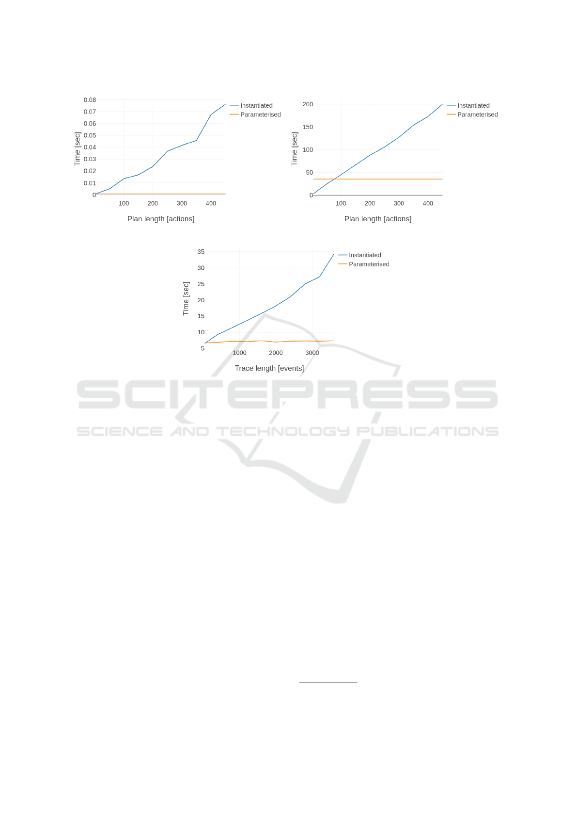
(a) Property synthesis. (b) Monitor synthesis.
(c) Runtime verification.
Figure 3: Results of experiments.
6 CONCLUSIONS
We have shown how to automatically synthesise mon-
itors to detect failures at runtime in a plan generated
by a classical planner. RVPLAN offers two methods
for generating monitors: based on instantiated actions
in the plan that the planner has sent as output; or based
on the actions in the domain specification. The former
is best when the plan’s length is not large; the latter is
more appropriate when the plan’s length is large but
there are not as many planning operators.
Note that the parameterised approach outperforms
the instantiated one, except for monitor synthesis. Be-
cause of this, none of the two can be considered the
best, in general. Instead, a hybrid combination could
be beneficial; where the instantiated approach is used
while the parameterised one is synthesising the mon-
itor. In this way, the time needed by the parame-
terised approach for synthesising a monitor can be
covered by the instantiated one. Upon synthesis com-
pletion, the instantiated monitor can be swapped with
its parameterised counterpart which, as experiments
showed, offers better verification performance.
As future work, we want to use the feedback gen-
erated by RVPLAN monitors to trigger replanning
and use information obtained during verification to
update the planning model. Initially, we are looking
into only updating the problem representation, that
is, updating the values of predicates that could have
changed and caused the plan to fail. Eventually, we
want to extend these monitors to also be able to aid
the planner in plan repair, not only updating the prob-
lem specification, but also reconfiguring action speci-
fications in the domain.
We also want to translate the effects of actions as
well, but this may require a logic that allows us to
define interval properties (such as Metric Temporal
Logic (Koymans, 1990)) and could benefit from us-
ing durative actions found in temporal planning. An-
other avenue for future work is to extend our theory
to include PDDL requirements such as disjunctive,
existential, universal, and quantified preconditions,
among others. Finally, we want to apply RVPLAN
to realistic case studies. For example, in robot appli-
cations developed in ROS
6
we could take advantage
6
https://www.ros.org/
ICAART 2022 - 14th International Conference on Agents and Artificial Intelligence
76

of the ROSMonitoring (Ferrando et al., 2020) tool to
generate our monitors for ROS applications.
ACKNOWLEDGEMENTS
Cardoso’s work supported by Royal Academy of En-
gineering under the Chairs in Emerging Technologies
scheme.
REFERENCES
Andreas Bauer, Martin Leucker, C. S. (2011). Runtime ver-
ification for LTL and TLTL. ACM Trans. Softw. Eng.
Methodol., 20(4):14:1–14:64.
Bartocci, E., Falcone, Y., Francalanza, A., and Reger, G.
(2018). Introduction to runtime verification. In Lec-
tures on Runtime Verification - Introductory and Ad-
vanced Topics, volume 10457 of Lecture Notes in
Computer Science, pages 1–33. Springer.
Bauer, A., Leucker, M., and Schallhart, C. (2010). Com-
paring LTL semantics for runtime verification. J. Log.
Comput., 20(3):651–674.
Bensalem, S., Havelund, K., and Orlandini, A. (2014). Ver-
ification and validation meet planning and scheduling.
Int. J. Softw. Tools Technol. Transf., 16(1):1–12.
Bozzano, M., Cimatti, A., Roveri, M., and Tchaltsev, A.
(2011). A comprehensive approach to on-board au-
tonomy verification and validation. In Walsh, T., edi-
tor, Proceedings of the 22nd International Joint Con-
ference on Artificial Intelligence, Barcelona, Catalo-
nia, Spain, July 16-22, 2011, pages 2398–2403. IJ-
CAI/AAAI.
Cardoso, R. C. and Bordini, R. H. (2019). Decentralised
planning for multi-agent programming platforms. In
Proceedings of the 18th International Conference on
Autonomous Agents and MultiAgent Systems, pages
799–807, Richland, SC. IFAAMAS.
Cashmore, M., Fox, M., Long, D., Magazzeni, D., Ridder,
B., Carreraa, A., Palomeras, N., Hurt
´
os, N., and Car-
rerasa, M. (2015). Rosplan: Planning in the robot op-
erating system. In ICAPS, page 333–341. AAAI Press.
Ferrando, A., Cardoso, R. C., Fisher, M., Ancona, D.,
Franceschini, L., and Mascardi, V. (2020). Ros-
monitoring: a runtime verification framework for ros.
In Towards Autonomous Robotic Systems Conference
(TAROS).
Fikes, R. E. and Nilsson, N. J. (1971). Strips: A new ap-
proach to the application of theorem proving to prob-
lem solving. Artificial Intelligence, 2(3):189 – 208.
Fox, M., Gerevini, A., Long, D., and Serina, I. (2006). Plan
stability: Replanning versus plan repair. In ICAPS,
volume 6, pages 212–221.
Frank, J. (2015). Reflecting on planning models: A chal-
lenge for self-modeling systems. In 2015 IEEE Inter-
national Conference on Autonomic Computing, pages
255–260.
Ghallab, M., Ingrand, F., Solange, L.-C., and Py, F. (2001).
Architecture and tools for autonomy in space. In
International Symposium on Artificial Intelligence,
Robotics and Automation in Space (ISAIRAS 2001).
Havelund, K., Peled, D., and Ulus, D. (2018). Dejavu: A
monitoring tool for first-order temporal logic. In 2018
IEEE Workshop on Monitoring and Testing of Cyber-
Physical Systems (MT-CPS), pages 12–13.
Havelund, K., Peled, D., and Ulus, D. (2020). First-order
temporal logic monitoring with bdds. Formal Methods
Syst. Des., 56(1):1–21.
Havelund, K. and Rosu, G. (2004). An overview of the run-
time verification tool java pathexplorer. Formal Meth-
ods Syst. Des., 24(2):189–215.
Kamp, H. (1968). Tense Logic and the Theory of Linear
Order. PhD thesis, Ucla.
Koymans, R. (1990). Specifying real-time properties with
metric temporal logic. Real Time Syst., 2(4):255–299.
Lichtenstein, O., Pnueli, A., and Zuck, L. D. (1985). The
glory of the past. In Logics of Programs, Conference,
Brooklyn College, New York, NY, USA, June 17-19,
1985, Proceedings, volume 193 of Lecture Notes in
Computer Science, pages 196–218. Springer.
Manna, Z. and Pnueli, A. (1989). Completing the tem-
poral picture. In Automata, Languages and Pro-
gramming, 16th International Colloquium, ICALP89,
Stresa, Italy, July 11-15, volume 372 of Lecture Notes
in Computer Science, pages 534–558. Springer.
Mart
´
ın, F., Gin
´
es, J., Rodr
´
ıguez, F. J., and Matell
´
an, V.
(2021). Plansys2: A planning system framework for
ros2. In IEEE/RSJ International Conference on Intel-
ligent Robots and Systems, IROS 2021, Prague, Czech
Republic, September 27 - October 1, 2021. IEEE.
Mayer, M. C. and Orlandini, A. (2015). An executable se-
mantics of flexible plans in terms of timed game au-
tomata. In 22nd International Symposium on Tempo-
ral Representation and Reasoning, TIME 2015, Kas-
sel, Germany, September 23-25, 2015, pages 160–
169. IEEE Computer Society.
Mayer, M. C., Orlandini, A., and Umbrico, A. (2016). Plan-
ning and execution with flexible timelines: a formal
account. Acta Informatica, 53(6-8):649–680.
Mcdermott, D., Ghallab, M., Howe, A., Knoblock, C., Ram,
A., Veloso, M., Weld, D., and Wilkins, D. (1998).
PDDL - The Planning Domain Definition Language.
Technical Report TR-98-003, Yale Center for Com-
putational Vision and Control.
Meneguzzi, F. and Luck, M. (2013). Declarative Planning in
Procedural Agent Architectures. Expert Systems with
Applications, 40(16):6508 – 6520.
Nau, D., Ghallab, M., and Traverso, P. (2004). Automated
Planning: Theory & Practice. Morgan Kaufmann
Publishers Inc., San Francisco, CA, USA.
Pnueli, A. (1977). The temporal logic of programs. In 18th
Annual Symposium on Foundations of Computer Sci-
ence, Providence, Rhode Island, USA, 31 October - 1
November, pages 46–57. IEEE Computer Society.
Sardina, S. and Padgham, L. (2011). A BDI Agent Pro-
gramming Language with Failure Handling, Declar-
ative Goals, and Planning. Autonomous Agents and
Multi-Agent Systems, 23(1):18–70.
RVPLAN: Runtime Verification of Assumptions in Automated Planning
77
