
Optimal 1-Request Insertion for the Pickup and Delivery Problem with
Transfers and Time Horizon
Jos
´
e-L. Figueroa, Alain Quilliot, H
´
el
`
ene Toussaint and Annegret Wagler
LIMOS INP, Universit
´
e Clermont Auvergne, France
fi
Keywords:
Pickup and Delivery Problem with Transfers, 1-Request Exact Insertion, Constrained Shortest Path, Constraint
Propagation, Time Expanded Networks.
Abstract:
In this paper, we deal with a subproblem of the Pickup and Delivery Problem with Transfers (PDPT) where
a finite set of transportation requests has been assigned to a homogeneous fleet of limited capacity vehicles,
while satisfying some constraints imposed by a set of pre-scheduled tours. Then, a new transportation request
appears, and we also have to serve it. For that, we can modify the current tours by performing a finite sequence
of changes allowing to pick up, transport, transfer or deliver this new request. The resulting tours must serve
all the requests and satisfy the original constraints, but within a given time horizon. To solve this problem, we
present an empirical Dijkstra algorithm that computes tentative solutions whose consistence is checked through
constraint propagation, and an exact algorithm which is an adaptation of the well-known A* algorithm for
robot planning, that performs an exhaustive search in a tree of partial solutions and reduces the combinatorial
explosion by pruning some unfeasible/redundant tree nodes. We conclude by comparing the performance of
both algorithms.
1 INTRODUCTION
In this first section, we give an informal description
of the problem that we are going to treat in this paper,
which is about the way that one additional request can
be inserted into the current solution of a pickup and
delivery instance, and we survey briefly some litera-
ture related to this problem which we call 1-Request
Insertion PDPT. This problem will be presented for-
mally in Section 2. In Section 3, we will describe two
algorithms for dealing with it. Finally, in Section 4
we compare the quality of the found solutions and the
performance of both algorithms over several data sets
of pseudorandom instances.
A standard Pick up and Delivery Problem (PDP)
most often involves a finite set V of identical vehi-
cles with capacity c, which must be scheduled in or-
der to perform a set of Pick and Delivery tasks inside
some network G. Time windows may be involved,
but, in most cases, a time horizon [0,T
max
] is imposed
for the whole schedule. Vehicles must meet a set R
of requests: a request r ∈ R consists in an origin o
r
, a
destination d
r
and a load ℓ
r
, and r has to be served
by exactly one vehicle. In the PDP with transfers
(PDPT), a request may be served by several vehicles,
in the sense that load ℓ
r
may start from origin o
r
with
some vehicle v
1
, and next shift to some vehicle v
2
at
some relay vertex x, and so on, until reaching destina-
tion d
r
into some vehicle v
p
. Depending on the con-
text, a transfer from v
1
to v
2
may take different forms:
one may impose either vehicles to meet (strong syn-
chronization constraint) at relay vertex x, or only for-
bid vehicle v
2
from leaving x before the arrival of v
1
(weak synchronization constraint). In other words, a
weak synchronization constraint implies that v
1
and
v
2
are obliged to meet only when v
2
arrives first to the
relay vertex x.
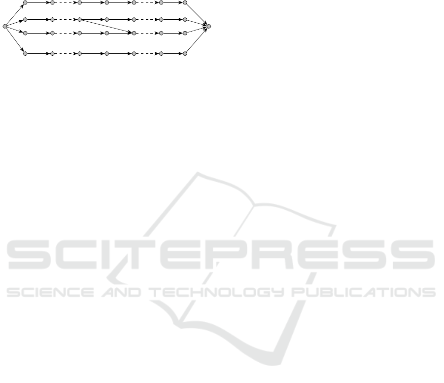
In this last case, a convenient way to model PDPT
is through the use of time expanded networks (see, for
example, (Gouveia et al., 2019) and (Bsaybes et al.,
2019)). We construct a network (see Figure 1) whose
vertex set consists of a dummy source vertex s, a
dummy sink vertex p, and a copy (x,t
i
) of every ver-
tex x of G and for any time value t
i
∈ [0,T
max
] (note
that in practice, we usually consider only a finite set
of relevant time values t
i
). We represent any feasible
move along an arc of G, from a vertex x to a vertex y
between time t
i
and time t
i
+δ (where δ ≥ 0), by some
arc
(x,t
i
),(y,t
i
+ δ)
. If x = y then such a move be-
comes a waiting move. Then, we represent vehicles
circulation by a unique integral flow vector F indexed
over the set A of the expanded network arcs, and re-
Figueroa, J., Quilliot, A., Toussaint, H. and Wagler, A.
Optimal 1-Request Insertion for the Pickup and Delivery Problem with Transfers and Time Horizon.
DOI: 10.5220/0010787000003117
In Proceedings of the 11th International Conference on Operations Research and Enterprise Systems (ICORES 2022), pages 17-27
ISBN: 978-989-758-548-7; ISSN: 2184-4372
Copyright
c
2022 by SCITEPRESS – Science and Technology Publications, Lda. All rights reserved
17
quests circulation comes as a multi-commodity flow
{ f
r
: A → R,r ∈ R}, such that for every arc a ∈ A of
the expanded network, the sum Σ
r∈R
f
r
(a) is less than
or equal to the value F
a
of vector F on arc a.
s
(y, 0)
(x, 0) (x, 1) (x, t
i
)
(y, t
i
+δ)
(x, T
max
)
(y, T
max
)
p
Figure 1: A Time Expanded Network.
Still, resulting models are not very well-fitted to
numerical handling, both because of their size and be-
cause PDP tends to arise in dynamic contexts, with re-
quests not completely known in advance, and which
must be managed in a flexible way. It comes that most
often, PDPT is handled in a heuristic way and a com-
mon strategy is to rely on an insertion (or build &
destroy) approach: requests are successively inserted
into some current schedule, and possibly removed and
reinserted in order to improve the related cost.
According to this paradigm, the key issue be-
comes the related insertion process. In case no trans-
fer is allowed, the insertion is trivial in the sense that
it can be performed through enumeration. It is not
the case when transfers are allowed. As a matter of
fact, inserting a request r becomes then significantly
more difficult than simply searching for some path
from origin o
r
to destination d
r
inside some ad hoc
network (or even time expanded network) because
synchronization (strong or weak) constraints require-
ments tend to impact the whole current schedule.
So the purpose of this work is to thoroughly study
the one request insertion problem that occurs as a
part of the Pickup and Delivery Problem with Trans-
fers (with time horizon), and that we will denote by
1-Request Insertion PDPT. We are first going to solve
it in an exact way, without imposing any restriction
neither on the number of transfers nor on the charac-
teristics on the transfer parameters, through a combi-
nation of constraint propagation techniques and an A*
like algorithm.
Let us recall that A* algorithm (see (Nilsson,
1980) or (Dechter and Pearl, 1985)) is an artificial in-
telligence oriented version of Dijkstra’s algorithm for
shortest path, designed in order to deal with huge net-
works whose nodes represent the possible states of a
system.
Next, in order to fit with the purpose of practical
use in realistic dynamic contexts, we shall describe a
heuristic algorithm, which also relies on the use of Di-
jkstra’s algorithm, augmented with a “closure” mech-
anism.
Finally, we shall observe the behavior of the algo-
rithms once we impose some common sense restric-
tions to the way that transfers can be performed.
Related Works
Surveys for Pickup and delivery problems can be
found, for example, in (Berbeglia et al., 2007),
(Berbeglia et al., 2010), and (Ho et al., 2018).
The notion of PDP with transfers was introduced
by (Laporte and Mitrovi
´
c-Mini
´
c, 2006) in the so-
called Pickup and Delivery Problem with Time Win-
dows and Transshipment, which is a PDP character-
ized for the presence of transshipment points, where
the vehicles can drop some objects or split their loads
to allow other vehicles to pick them up later.
An exact method for some PDPT was presented
by (Contardo et al., 2010). In their paper, the authors
construct a complex mixed-integer linear program-
ming formulation, and they confirm that it works cor-
rectly by solving an example instance with a method
based on Benders decomposition.
In (Bouros et al., 2011), the authors address the
dynamic PDPT and propose a graph-based formu-
lation that treats each request independently as a
constrained shortest path problem. They compare
this approach against a relatively conventional local
search algorithm based on insertion heuristics and
tabu search, and conclude that their method is sig-
nificantly faster with the inconvenience that solutions
quality is marginally lower.
The computational complexity of checking the
feasibility for the insertion of one request in the PDPT
was studied by (Lehu
´
ed
´
e et al., 2013). In this work,
the authors determined that if we perform some pre-
processing of the current state of a PDPT network,
we can test the feasibility of insertions in constant
time, and the complexity to update the preprocessed
information after insertion/deletion of one request is
quadratic in the size of the network.
Above-mentioned contributions (Bouros et al.,
2011) and (Lehu
´
ed
´
e et al., 2013) are the closest ones
to our contribution. Both rely on the construction of
auxiliary graphs, which represent the current state of
vehicle paths together with some specific constraints
related to transfers. Still (Bouros et al., 2011) does
not care of time’s feasibility (i.e. time windows) nor
the impact of restrictions imposed to the transfers.
At the opposite, (Lehu
´
ed
´
e et al., 2013), is a theoret-
ical contribution which focuses on the complexity of
testing the feasibility of an insertion (with one trans-
fer at most), after some preprocessing that allows the
management of slack time variables. Our contribu-
tion lays in between: while we also rely on precom-
ICORES 2022 - 11th International Conference on Operations Research and Enterprise Systems
18

putation of length path values, we relax the restric-
tions on the transfer vertices, impose no restriction on
the number of transfers, and propose both exact and
heuristic algorithms for the computation of a best fea-
sible insertion for a given request. Then we analyze
through numerical experiments, the impact on both
the behavior of the algorithms and the nature of the
solutions.
2 FORMAL MODEL
We first suppose that we are provided with a finite set
X of “points” representing physical locations, given
together with:
• A distance function d : X × X → R
+
, such that
for any x,y ∈ X, the value d(x,y) means the time
required for a vehicle to move in X from x to y
according to a shortest path strategy.
• A function µ : X × X → X is going to be involved
in order to determine “relay vertices”, that means
the points where two vehicles v
1
, v
2
will meet in
order to perform some transfer. Intuitively, for
any (x
1
,x
2
) ∈ X × X, the element u = µ(x
1
,x
2
)
corresponds to a place that is more or less at
the same distance from x to y and minimizes the
sum d(x
1
,u) + d(u,x
2
). For example, if X con-
tains points from a Euclidean space, we can define
u = µ(x
1
,x
2
) as an element in X with minimal dis-
tance to the midpoint of the segment from x
1
to x
2
.
2.1 PDPT Problem
A PDPT instance consists of a finite set of points X
together with the two functions d : X × X → R
+
and
µ : X × X → X that we have just defined, a finite set
of vehicles V with a homogeneous capacity c ∈ R
+
, a
time horizon [0,T
max
], and a finite set R ⊂ X ×X × R
+
of requests r = (o
r
,d
r
,ℓ
r
). The point o
r
is the origin
of r, the point d
r
is the destination of r, and ℓ
r
is the
load of r. Also, each vehicle v ∈ V has assigned two
distinguished points: one starting depot point D
v
s
∈ X
and one ending depot point D
v
e
∈ X. Figure 2 shows
an example of PDPT instance.
Now we will briefly describe the PDPT. We are
not going to deal here with the whole problem, how-
ever, for completeness reasons it is important to give
at least some intuition and clarify some details in-
volved. This will set the stage later to present our
formal model for the insertion subproblem.
The PDPT consists in finding a schedule for the
vehicles fleet, allowing to transport the requests from
their origins to their destinations. Vehicles capac-
B
C
D
EA
A B C D E
A 0 1 2 2 1
B 1 0 1 2 2
C 2 1 0 1 2
D 2 2 1 0 1
E 1 2 2 1 0
A B C D E
A A A B E A
B A B B C A
C B B C C D
D E C C D D
E A A D D E
(a) (b)
(e)
(c)
(d)
X ={A,B,C,D, E}
V = {v, w}, c = 10, T
max
= 15,
D
s
v
= D
v
e
= D
s
w
= D
e
w
= A
R=
r
1
=(o
r
1
=B,d
r
1
=D,`
r
1
=5),
r
2
=(o
r
2
=D,d
r
2
=B,`
r
2
=2)
Figure 2: An example of PDPT instance. (a) The set X =
{A,B,C, D, E} of points. (b) A symmetric matrix whose
entries define the distance function d. (c) A matrix defining
the function µ. (d) The set of vehicles V = {v, w}, the capac-
ity c, the upper limit of the time horizon [0, T
max
], and the
starting and ending depot points of vehicles. (e) The set R
of requests consisting of r
1
= (B, D, 5) and r
2
= (D, B, 2).
ity must be respected at any moment, however, vehi-
cles are allowed to transfer requests to other vehicles
through a weak synchronization mechanism. This is,
if a vehicle v is transferring a load ℓ
r
to another vehi-
cle w at a relay vertex z, and the receiving vehicle w
arrives first to z, then w has to wait for the arriving of v
with the load ℓ
r
. The time duration for traversing ev-
ery path in the schedule (considering waiting times),
must be within the given time horizon.
Depending on the context, there can be several
ways to define the cost of such schedules. Here, we
put the focus on the point of view of the users, and
consider that the cost of a schedule is the sum of
the distances traversed by the requests, and then we
aim to find a minimal cost schedule. This choice is
not particularly restrictive because the algorithms that
we will present can be adapted to handle other types
of costs (e.g. total mileage covered by the vehicles/
requests, or the time when they achieve their respec-
tive trips).
In the following subsection, we proceed to de-
scribe our formal model for the insertion problem in-
volved in the PDPT.
2.2 Formal Description of a PDPT
Feasible Solution
Let G
X
be the directed graph whose set of vertices is
X and whose set of arcs is {(x,y) ∈ X × X, x ̸= y}.
According to the above definition of a PDPT in-
stance, we define a solution (Γ,Π) for the PDPT in-
stance, which we also call a PDPT schedule as
• A collection Γ =
Γ(v), v ∈ V
of paths on G
X
,
where Γ(v) = (x
v
0
,x
v
1
,.. .,x
v
|Γ(v)|−1
) is the path fol-
lowed by vehicle v in G
X
.
Optimal 1-Request Insertion for the Pickup and Delivery Problem with Transfers and Time Horizon
19
• A collection Π =
Π(r), r ∈ R
, of paths on G
X
.
The directed path Π(r) = (y
r
0
,y
r
1
,.. .,y
r
|Π(r)|−1
) is
the path followed by load ℓ
r
when moving from
its origin o
r
to its destination d
r
. Points y
r
q
belong
to the set
x
v
i
: v ∈ V,0 ≤ i ≤ |Γ(v)| − 1
and we
may distinguish two classes of moves for request
r
– If y
r
q
and y
r
q+1
are related to two consecutive
vertices of path Γ(v), then they have to be con-
secutive in Π(r) and so we talk about vehicle
move inside vehicle v.
– If y
r
q
= x
v
i
and y
r
q+1
= x
w
j
are related to two dis-
tinct paths Γ(v) and Γ(w), then they refer to the
same vertex in X, and so we talk about transfer
move from vehicle v to vehicle w.
Denoting by X(Γ) the set
(v,i) : v ∈ V, 0 ≤ i ≤
|Γ(v)|−1
, we see that such a solution induces an ori-
ented graph structure G(Γ,Π) on the vertex set X(Γ),
with arc set A(Γ,Π) defined as follows
• With any v ∈ V and any 0 ≤ i ≤ |Γ(v)| − 1, we
associate a vehicle arc e = ((v, i), (v,i + 1)), with
length d
G
(e) = d(x
v
i
,x
v
i+1
). Following paths Π(r)
allows the computation of the load ℓ
v
i
of this arc,
which is the sum of loads ℓ
r
for requests r which
move through this arc. Of course ℓ
v
i
does not have
to exceed the capacity c (Load Constraints).
• With any r ∈ R and 1 ≤ q ≤ |Π(r)| − 1, such that
moving from y
r
q
= x
v
i
to y
r
q+1
= x
w
j
corresponds
to a transfer move from vehicle v to vehicle w,
we associate a transfer arc e = ((v,i), (w, j)), with
length d
G
(e) = d(y
r
q
,y
r
q+1
) = 0 (because in this
case, y
r
q
and y
r
q+1
correspond to the same place).
We denote by A
′
the set of those transfer arcs.
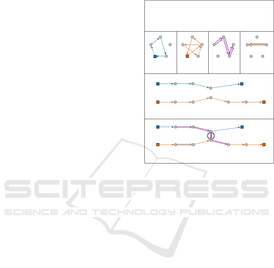
Figure 3 shows an example of solution (Γ,Π) for
the instance defined in Figure 2, and the associated
graph G(Γ,Π).
Feasibility of (Γ,Π): As we just told, (Γ, Π) must
meet the above Load Constraints. Also it must satisfy
time consistency constraints defined as follows:
• With any vertex (v, i) in the graph G(Γ,Π) we as-
sociate a time value t
v
i
which represents the ear-
liest time when vehicle v may leave vertex (v, i).
Then we see that
– For any vehicle arc ((v,i), (v,i + 1)), we have
that t
v
i+1
≥ t
v
i
+ d(x
v
i
,x
v
i+1
).
– Weak synchronization implies that t
w
j
≥ t
v
i
for
any transfer arc ((v, i),(w, j)).
They can be summarized as: (E1: Time Consistency
Constraints)
• For any arc e = ((v, i),(w, j)) in the graph
G(Γ,Π), we have that t
w
j
≥ t
v
i
+ d
G
(e).
(a)
B
C
D
A E
(b)
(c)
(d) (e)
(f)
(g)
arc in A
0
(w,0) (w,1) (w,2) (w,4) (w, 5) (w,6)
(v,0) (v,1) (v, 2)
(w,3)
=
=
Π(r
1
)
Γ =
Γ(v) = (x
v
0
= A, x
v
1
= B, x
v
2
= C, x
v
3
= E, x
v
4
= A),
Γ(w) = (x
0
w
= A, x
1
w
= D, x
2
w
= B, x
3
w
= E, x
4
w
= D, x
5
w
= C, x
6
w
= A)
Π =
Π(r
1
) = (y
r
0
1
= x
v
1
, y
r
1
1
= x
v
2
, y
r
2
1
= x
v
3
, y
r
3
1
= x
3
w
, y
r
4
1
= x
4
w
),
Π(r
2
) = (y
r
0
1
= x
1
w
, y
r
1
2
= x
2
w
)
B
C
D
A E
B
C
D
A E
B
C
D
A E
Γ(v)
Γ(w)
Π(r
2
)
(v,0) (v,1) (v, 2)
(w,0) (w,1) (w,2)
(w,3)
(w,4) (w,5) (w,6)
Γ(v)
Γ(w)
y
r
0
1
= o
r
1
y
r
1
1
y
r
1
2
y
r
0
2
y
r
1
3
d
r
1
= y
r
4
1
= o
r
2
d
r
2
= y
r
1
2
Π(r
2
)
Π(r
1
)
5
5
(v,3)
(v,3)
(v,4)
(v,4)
2
5
Figure 3: (a) An example of solution for the instance de-
fined in Figure 2. (b)-(e) Subgraphs of G
X
edge-induced
by the paths Γ(v), Γ(w), Π(r
1
) and Π(r
2
), respectively.
(f) The paths on the directed graph G(Γ,Π) correspond-
ing to the directed paths Γ(v) and Γ(w) of G
X
. (g) The
directed graph G(Γ, Π). We have also depicted with dou-
ble arrows the directed paths corresponding to Π(r
1
) and
Π(r
2
). Numbers indicate positive loads traversing through
arcs in A(Γ,Π) \ A
′
.
• Due to the time horizon [0,T
max
], for any (v,i) we
have that 0 ≤ t
v
i
≤ T
max
.
They impose that: (E2: No Cycles Constraint)
• Arc set A(Γ, Π) does not contain any cycle.
If (Γ,Π) satisfies those constraints, we can asso-
ciate, with every (v,i) in G(Γ, Π), some time windows
[Min
v
i
, Max
v
i
] related to variables t
v
i
, constrained by
(E1).
Cost of a Solution (Γ, Π): As we said in 2.1, we
are going to define the cost of a solution as the sum of
the distances traversed by the requests.
2.3 The 1-Request Insertion PDPT
Model
Those preliminaries allow us to define in a formal way
the 1-Request Insertion PDPT, about the insertion of
a new request into a current feasible PDPT schedule
(Γ,Π). So we start from such a feasible schedule
(Γ,Π), and from an additional request r = (o
r
,d
r
,ℓ
r
).
ICORES 2022 - 11th International Conference on Operations Research and Enterprise Systems
20
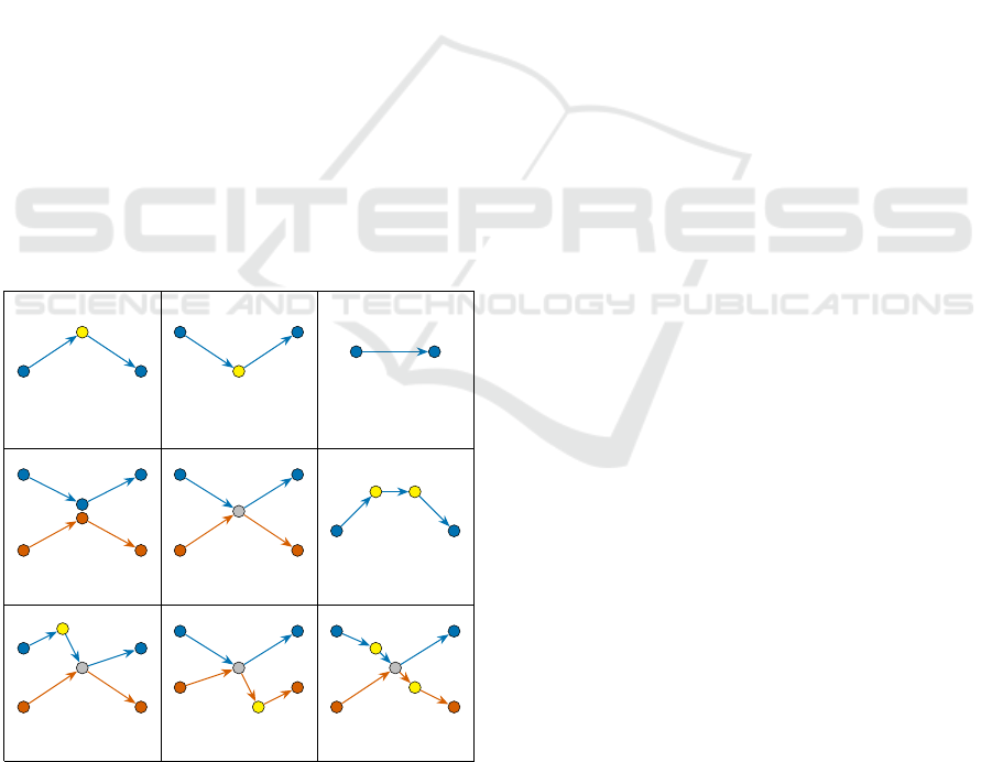
Intuitively, inserting request r means building a suit-
able sequence of the following five types of moves:
(1) Start from o
r
and enter into some path Γ(v) at the
level of some vertex (v, i + 1), and so imposing
vehicle v to make a deviation between (v,i) and
(v,i + 1). Such a move will be performed once as
the initial move (See Figure 4 (a)).
(2) Leave some path Γ(w) at the level of some vertex
(v,i) in order to reach d
r
, and so impose a vehicle
to make a deviation between (v, i) and (v,i + 1).
Such a move will be performed once as the final
move (See Figure 4 (b)).
(3) Keep on inside vehicle v, while moving from
some (v,i) to its successor (v, i + 1). Such a type
of move will be possibly performed several times
(See Figure 4 (c)).
(4) Move from vehicle v to vehicle w while using
some arc ((v, i),(w, j)) of A
′
and some shared
point x
v
i
= x
w
j
. Such a type of move will be possi-
bly performed several times (See Figure 4 (d)).
(5) Move from vehicle v to vehicle w while getting
out of v while running between some vertex (v, i)
and its successor and entering into w at the level
of some vertex (w, j), and while w is moving from
(w, j − 1) to its successor. Such a move will be
possibly performed several times (See Figure 4
(e)).
(v, i) (v, i + 1)
o
r
(v, i) (v, i + 1)
d
r
(v, i) (v, i + 1)
(v, i − 1)
(v, i)
(v, i + 1)
x
i
v
= x
j
w
(w, j − 1)
(w, j)
(w, j + 1)
(v, i) (v, i + 1)
z
(w, j − 1) (w, j)
(v, i) (v, i + 1)
o
r
d
r
(v, i) (v, i + 1)
o
r
z
(w, j − 1) (w, j)
(v, i) (v, i + 1)
z
(w, j − 1) (w, j)
d
r
(v, i) (v,i + 1)
o
r
z
d
r
(w, j − 1) (w, j)
(a) (b) (c)
(d) (e) (f)
(g) (h) (i)
Figure 4: Types of vehicle’s moves for transporting a re-
quest r = (o
r
,d
r
,ℓ
r
).
Remark: For simplicity, in this work we are go-
ing to restrict our study to these 5 types of moves.
However, we note that it is also possible to combine:
(6) moves of types (1) and (2), in such a way that r
is inserted through a simple deviation of a vehicle
v between two successive vertices of Γ(v). This
is, while traversing Γ(v), vehicle v performs a de-
viation from (v,i) to transport the load ℓ
r
from o
r
directly to d
r
, and then v returns to its original path
at the level of vertex (v,i + 1) (See Figure 4 (f)).
(7) movements of types (1) and (5), in such a way
that, request r starts from o
r
in a vehicle v and
then is transferred directly to another vehicle w at
some relay vertex z, while v is moving from (v, i)
to (v,i +1), and while w is moving from (w, j − 1)
to (w, j) (See Figure 4 (g)).
(8) movements of types (2) and (5), in such a way
that r leaves some path Γ(v) (at the level of a ver-
tex (v,i)), to be transferred from v to w at some
relay vertex z. Then r reaches d
r
directly from z
in vehicle w. The first part of this process happens
while v is moving from (v, i) to (v, i + 1), and the
second one while w is moving from (w, j − 1) to
(w, j) (See Figure 4 (h)).
(9) moves of types (1), (2) and (5), in such a way that
r starts from o
r
in a vehicle v, then r is transferred
directly to another vehicle w at some relay vertex
z, and finally r reaches d
r
directly from z inside
vehicle w, while v is moving from (v, i) to (v, i +
1), and while w is moving from (w, j − 1) to (w, j)
(See Figure 4 (i)).
While moves of types 1, 2, 3, and 4 are easy to
understand, we need to better explain the moves of
type 5. Clearly, a move of type 5 involves some relay
vertex z: both vehicle v and w are going to perform a
deviation through z, vehicle v will drop load ℓ
r
in z,
and vehicle w will take it as soon as possible. In order
to identify z, we use function µ and we take:
z = µ
µ(x
v
i
,x
w
j
),µ(x
v
i+1
,x
w
j−1
)
. (E3)
Please notice that (E3) restricts our freedom to
choose the relay vertex, and so it has to be considered
as a hypothesis of the model.
Now, given a PDPT schedule (Γ,Π) and one ad-
ditional request r, we define the following graph
H(Γ,Π,r)
• Vertices of H(Γ,Π,r) are vertices of G(Γ, Π),
plus two vertices o
r
and d
r
.
• Arcs of H(Γ,Π, r) are
– In-arcs: they have the form e = (o
r
,(v,i)), with
0 ≤ i < |Γ(v)| − 1, length d
H
(e) = d(o
r
,x
v
i+1
),
and such that ℓ
v
i
+ ℓ
r
≤ c.
– Out-arcs: with the form e = ((w, j), d
r
), with
1 ≤ j ≤ |Γ(w)| − 1, length d
H
(e) = d(x
w
j
,d
r
),
and such that ℓ
w
j
+ ℓ
r
≤ c.
Optimal 1-Request Insertion for the Pickup and Delivery Problem with Transfers and Time Horizon
21
– Vehicle-arcs: arcs e = ((v, i),(v,i + 1)) in
G(Γ,Π), with length d
H
(e) = d
G
(x
v
i
,x
v
i+1
), and
such that ℓ
v
i
+ ℓ
r
≤ c.
– A
′
-arcs: the arcs e = ((v,i),(w, j)) ∈ A
′
, with
length d
H
(e) = d
G
(e) = 0.
– Transfer-arcs: with the form e = ((v,i), (w, j)),
length d
H
(e) = d(x
v
i
,z) + d(z,x
w
j
) where z is
defined as in (E3). These arcs are such that
ℓ
v
i
+ ℓ
r
≤ c and ℓ
w
j−1
+ ℓ
r
≤ c.
Let π be a path from o
r
to d
r
in H(Γ,Π,r). Note
that π may be interpreted as a sequence of moves
of types (1, ... ,5) allowing to transport the request
r from o
r
to d
r
.
If t
v
i
denotes the time when vehicle v leaves vertex
(v,i), then every in-arc, out-arc and transfer-arc of π
is going to impose additional constraints, to be added
to constraints (E1)
• An in-arc
o
r
,(v,i)
imposes one additional con-
straint t
v
i+1
≥ t
v
i
+ d(x
v
i
,o
r
) + d(o
r
,x
v
i+1
). (E4)
• An out-arc
(w, j), d
r
imposes one additional
constraint t
w
j+1
≥ t
w
j
+d(x
w
j
,d
r
)+d(d
r
,x
w
j+1
). (E5)
• A transfer-arc
(v,i),(w, j)
imposes three addi-
tional constraints (here, z is taken as in (E3) )
1. t
v
i+1
≥ t
v
i
+ d(x
v
i
,z) + d(z, x
v
i+1
). (E6.1)
(Deviation for vehicle v)
2. t
w
j
≥ t
w
j−1
+ d(x
w
j−1
,z) + d(z, x
w
j
). (E6.2)
(Deviation for vehicle w)
3. t
w
j
≥ t
v
i
+ d(x
v
i
,z) + d(z, x
w
j
). (E6.3)
(Weak Synchronization)
(E6)
Then a path π in H(Γ,Π, r) is going to be time-
consistent if it allows the existence of time vectors
t
v
= (t
v
0
,.. .,t
v
|Γ(v)|−1
), v ∈ V , which meet constraints
(E1) and additional constraints (E4, E5, E6) related to
π. Notice that if π is given, checking the time con-
sistence of π can be performed through a simple con-
straint propagation process.
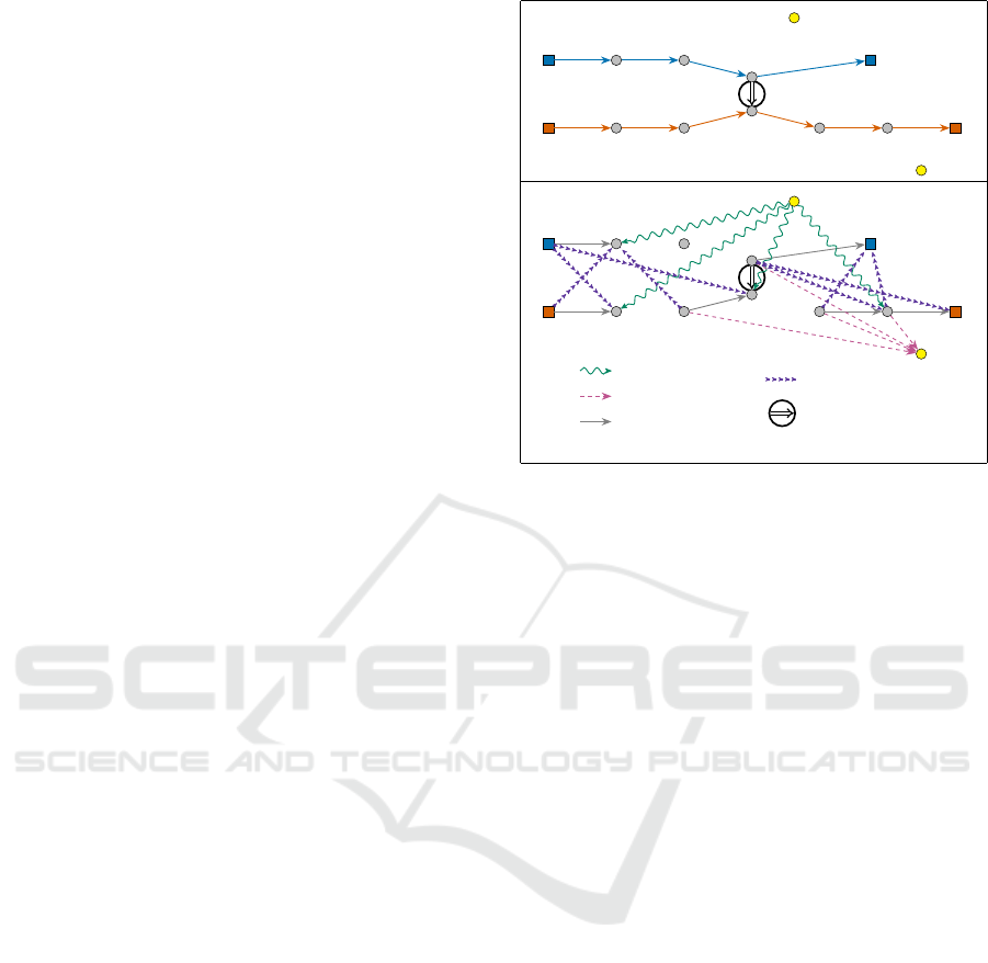
Figure 5 shows an example of construction of the
graph H(Γ,Π, r) from a PDPT schedule (Γ,Π) and
one additional request r = (o
r
,d
r
,ℓ
r
).
The 1-Request Insertion PDPT can be summa-
rized as follows:
1-Request Insertion PDPT: Given a PDPT sched-
ule (Γ, Π) and one request r = (o
r
,d
r
,ℓ
r
), compute
a shortest (in the sense of length function d
H
) time-
consistent path π from o
r
to d
r
in the graph H(Γ,Π,r).
Legend
In-Arc
Out-Arc
Vehicle-Arc
(a)
(b)
(v,0) (v,1) (v,2)
(v,3)
(v,4)
(w,0) (w,1)
(w,3)
(w,4) (w,5) (w,6)
o
r
d
r
0
5
5
0
0 2
0
5
0 0
arc in A
0
(v,0) (v,1)
(v,2)
(v,3)
(v,4)
(w,0) (w,1)
(w,2)
(w,3)
(w,4)
(w,5)
(w,6)
o
r
d
r
Transfer-arc
A
0
-arc
(w,2)
Figure 5: Deriving graph H(Γ,Π,r) from the PDPT sched-
ule (Γ, Π) corresponding to Figure 3, and one additional
request r = (o
r
= D, d
r
= B, ℓ
r
= 9). (a) The graph G(Γ,Π)
and the additional request r = (o
r
,d
r
,ℓ
r
). (b) The graph
H(Γ,Π, r). Notice that the capacity requirement forbids
some vehicle-arcs of G(Γ,Π).
3 ALGORITHMS
We are first going to work (in 3.1 and 3.2) con-
sidering all the transfers-arcs with enough capac-
ity to handle the given request. However, we can
notice that the number of transfer-arcs increases as
∑
v,w∈V,v̸=w
|Γ(v)| · |Γ(w)|, and then we shall adapt
in 3.3 the algorithms described in 3.1 and 3.2 in
such a way that they consider only well-fitted eligi-
ble transfer-arcs.
3.1 An Exact A*-like Algorithm
The A* algorithm was introduced in (Hart et al.,
1968) as an adaptation of Dijkstra’s algorithm in order
to deal with search path in very large state networks,
like those that one may have to handle in robotics. It
is our case here since at any time during the resolution
process, we shall deal not only with a current vertex
(v,i) of the graph H(Γ,Π, r), but also with time win-
dows related to vectors t
v
, v ∈ V .
We suppose that we are provided, as consequence
of some constraint propagation preprocess, with
• For any pair
(v,i),(w, j)
of vertices of G(Γ,Π),
the length Φ
(v,i),(w, j)
of a longest path
from (v,i) to (w, j) in the graph G(Γ,Π); vari-
ables t
v
i
and t
w
j
are constrained by t
w
j
≥ t
v
i
+
Φ
(v,i),(w, j)
.
ICORES 2022 - 11th International Conference on Operations Research and Enterprise Systems
22

• For any vertex u in the graph H(Γ,Π, r), the
length ω
u
of a shortest path from u to destination
vertex d
r
in H(Γ,Π,r). In case u ∈ V (Γ(v)) for
some v ∈ V we are also provided with a time win-
dow [Min
v
i
, Max
v
i
] derived from constraints (E1).
Then, as in standard A*, we perform a Breadth
First Search (BFS) process, driven by some list LS of
states, according to the algorithmic scheme described
in Algorithm 1.
Algorithm 1: A* 1-PDPT algorithmic scheme.
input : Graph H(Γ,Π,r), request
r = (o
r
,d
r
,ℓ
r
).
output: A time-consistent (o
r
, d
r
)-path with
best cost or a failure message.
1 LS ←{(o
r
,0,0, 0, Nil)} [Initialize LS] ;
2 Success ← False ;
3 while LS Not empty and Not Success do
4 (u,λ, δ, ω, S )←Head(LS) [Current state];
5 Remove Head(LS) from LS;
6 if u ̸= d
r
then
7 Expand current state (u, λ, δ, ω, S ) (I1);
8 else
9 Success ← True;
10 end
11 end
12 if Not Success then
13 Print “No path found”;
14 else
return: Path retrieved from current state.
15 end
State’s Definition: Every element s of LS is a
state, that means a 5-uple s = (u,λ,δ, ω,S ), where
• u is a vertex of the graph H(Γ,Π, r).
• λ ∈ R is the value of the current length of the path
π(u) from origin o
r
to u which has been achieved.
• δ ∈ R is a lower bound on the arriving time to u. In
case u = (v,i) ∈ V (Γ(V )) for some v ∈ V , we will
write δ
v
i
instead of δ; feasibility of state s implies
that Min
v
i
≤ δ
v
i
≤ Max
v
i
.
• ω ∈ R is the sum ω
u
+λ, that is a lower bound for
any path π which would extend current path π(u);
LS remains sorted in increasing order according to
ω values.
• S is a list of transfer-arcs
(v,i),(w, j)
which
have been involved in π(u), together with lower
bounds δ
v
i
,δ
v
i+1
,δ
w
j−1
,δ
w
j
, on t
v
i
, t
v
i+1
, t
w
j−1
, and t
w
j
,
respectively.
Domination Rule: Let π(u) and π(u
′
) be time-
consistent paths retrieved from two different states
s = (u,λ,δ, ω,S ) and s
′
= (u
′
,λ
′
,δ
′
,ω
′
,S
′
), respec-
tively. For any v ∈ V , let t
v
s
, t
v
s
′
, respectively, be
the lexicographically smallest time vectors (meeting
E1 and E4-E6) related to π(u) and π(u
′
). Let V
u
=
{v ∈ V : V (π(u)) ∩ V (Γ
v
) ̸=
/
0} and V
u
′
= {v ∈ V :
V (π(u
′
)) ∩V (Γ
v
) ̸=
/
0}.
We say that the state s dominates the state s
′
if u =
u
′
, λ < λ
′
, δ ≤ δ
′
, V
u
⊆ V
u
′
and for all v ∈ V
u
∩V
u
′
we
have that max{ j : (v, j) ∈ V (π(u))} ≤ max{ j : (v, j) ∈
V (π(u
′
))}, and for every v ∈ V we have that t
v
s
≤ t
v
s
′
.
This rule can be used to remove some redundant states
when we are exploring the BFS tree of states.
Expand Mechanism (I1) : Expanding state s =
(u,λ,δ, ω,S ), means consider the arcs e = (u, v) of
H(Γ,Π,r) with tail u and, for any such an arc, com-
puting resulting state s
′
e
= (v,λ
′
= λ + d(e), δ
′
,ω
′
=
λ
′
+ ω
v
,S
′
), where δ
′
and S
′
derive from δ and S ,
respectively, after propagation of constraints E1, E4,
E5, E6. If the path π(v), retrieved from s
′
e
, is time-
consistent and s
′
e
is not dominated by any state in LS,
then we insert s
′
e
into LS and possibly remove from
LS any state dominated by s
′
e
. Note that, the con-
straint propagation mechanism which yields δ
′
and S
′
is induced by the transfer-arcs which have been used
in order to reach u, and which are contained into the
list S .
Figure 6 contains a representation of a state from
a list LS and gives some intuition about the expanding
mechanism (I1).
Now, we note that
• The A* algorithm performs an exhaustive search
on the tree of states corresponding to time-
consistent paths.
• A path which is not time-consistent cannot be ex-
tended into a time-consistent one.
• The domination rule removes only redundant
states.
Hence we have the following.
Proposition 1. Above A* 1-PDPT solves 1-Request
Insertion PDPT in an exact way (taking into account
the (E3) hypothesis), in a time which does not exceed
O
∆
+
(H(Γ,Π,r))
m+1
· Size(H(Γ,Π, r))
where
∆
+
(H(Γ,Π,r)) is the maximum outdegree of a vertex
in H(Γ,Π,r), and where m is the maximum number
of arcs in a path π(u) retrieved from a state s = (u, λ,
δ, ω, S ) that was involved in LS.
Remark: The complexity of the 1-Request Inser-
tion PDPT remains an issue. Still, in the case we
impose a small constant (e.g. 3 or 5) as a bound on
the number of transfer-arcs of the constructed paths,
a simple counting argument can show that it becomes
time-polynomial.
Optimal 1-Request Insertion for the Pickup and Delivery Problem with Transfers and Time Horizon
23
(v
1
,0) (v
1
,1) (v
1
,2) (v
1
,3) (v
1
,4)
(v
2
,0) (v
2
,1)
(v
2
,2)
(v
2
,3) (v
2
,4) (v
2
,5)
(v
3
,0) (v
3
,1) (v
3
,2)
(v
3
,3)
(v
3
,4)
(v
4
,0) (v
4
,1) (v
4
,2)
(v
4
,3)
(v
4
,4)
o
r
d
r
(v
3
,5)(v
3
,6)
S =
(v
1
,2),(v
2
,2)
,
(v
2
,4),(v
3
,3)
,
δ
v
2
1
, δ
v
3
1
, δ
v
1
2
, δ
v
2
2
, δ
v
4
2
, δ
v
5
2
, δ
v
2
3
, δ
v
3
3
Γ(v
1
)
Γ(v
2
)
Γ(v
3
)
Γ(v
4
)
Figure 6: Representation of a particular state s =
u =
(v
3
,4),λ, δ, ω, S
from a list LS. Bold arcs indicate the cor-
responding path π(u) from origin o
r
to u which has been
achieved. The information stored in S allow us to determine
which vertices are involved in path π(u), and also give us
estimations for the arriving times to those vertices. Dashed
arcs allow extending the current path π(u), so they corre-
spond to new states that can be derived from s via the ex-
panding mechanism (I1).
3.2 A Practical Dijkstra-like Algorithm
Since our problem is likely to arise in a dynamic con-
text, we must try to propose approaches which are less
time consuming than the previous one. In order to
do it, we fix some integer parameter m > 0, and next
for every (v,i) with v ∈ V , i ∈ {0,. . .,|Γ(v)| − 1}, we
compute shortest paths π(v,i), in the graph H(Γ,Π, r),
from vertex (v,i) to destination d
r
, while using Di-
jkstra’s algorithm (see Figure 7 (a)). We denote by
ω(v,i) the length of π(v,i). Notice that such computa-
tions are involved in A* 1-PDPT algorithm, in order
to provide us with ω values involved in Algorithm 1.
Then, we close those computed paths π(v,i)
(see Figure 7 (b)) to obtain (o
r
, d
r
)-paths π
∗
(v,i) =
(o
r
,(v,i)) + π(v, i) (i.e. we create a path from o
r
to d
r
whose first arc is the in-arc (o
r
,(v,i)) and
the remaining arcs are the ones of path π(v, i)).
For each constructed path π
∗
(v,i), we compute the
value d
o
r
,(v,i)
+ ω(v,i), and then we select the m
paths π
∗
(v
1
,i
1
),.. .,π
∗
(v
m
,i
m
) with the lowest values
d
o
r
,(v,i)
+ ω(v, i). Finally, we check for every se-
lected path π
∗
(v
k
,i
k
), 1 ≤ k ≤ m, the consistence of
the additional constraints induced by the in-arc, the
out-arc and the transfer-arcs of π
∗
(v
k
,i
k
), and we keep
the path π
∗
which meets this consistence test and
which is related to the smallest d
o
r
,(v,i)
+ ω(v, i)
value. This process is summarized in Algorithm 2.
(a)
(b)
o
r
o
r
(v
1
,0)
(v
1
,1)
(v
1
,2) (v
1
,3) (v
1
,4)
(v
2
,0)
(v
2
,1)
(v
2
,2) (v
2
,3) (v
2
,4) (v
2
,5)
(v
3
,0) (v
3
,1) (v
3
,2)
(v
3
,3)
(v
3
,4) (v
3
,5)(v
3
,6)
(v
4
,0) (v
4
,1)
(v
4
,2)
(v
4
,3) (v
4
,4)
d
r
Γ(v
1
)
Γ(v
2
)
Γ(v
3
)
Γ(v
4
)
(v
1
,0)
(v
1
,1)
(v
1
,2) (v
1
,3) (v
1
,4)
(v
2
,0)
(v
2
,1)
(v
2
,2) (v
2
,3) (v
2
,4) (v
2
,5)
(v
3
,0) (v
3
,1) (v
3
,2)
(v
3
,3)
(v
3
,4) (v
3
,5)(v
3
,6)
(v
4
,0) (v
4
,1)
(v
4
,2)
(v
4
,3) (v
4
,4)
d
r
Γ(v
1
)
Γ(v
2
)
Γ(v
3
)
Γ(v
4
)
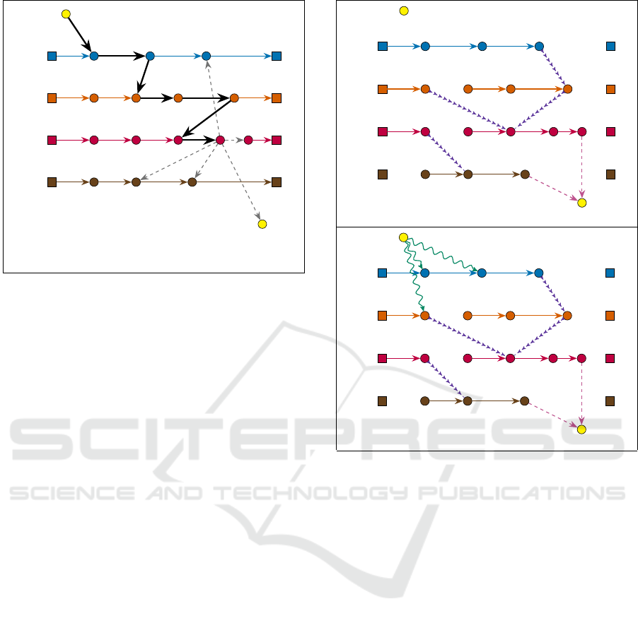
Figure 7: Deriving solutions from a Dijkstra’s shortest path
computation. (a) A subgraph Ψ of a graph H(Γ,Π, r) ob-
tained by Dijkstra’s algorithm while computing a shortest
path π(v, i) from every vehicle vertex (v, i) to d
r
. (b) Graph
Ψ is extended by adding some in-arcs from H(Γ, Π, r)
(wavy arrows). Every path from o
r
to d
r
in the resulting
graph gives rise to a solution for handling request r, and the
time feasibility of such a solution is then checked through
constraint propagation.
3.3 Controlling Transfer-arcs Number
As mentioned at the beginning of Section 3, the num-
ber of transfer-arcs is an issue, since most arcs of
H(Γ,Π,r) are transfer-arcs, while at the end, the best
time-consistent paths usually contain very few of such
arcs. In order to deal with the number of transfer-arcs
issue, we impose to transfer-arcs some eligibility re-
quirement, which depends on a threshold parameter
ε ≥ 0.
ε-eligibility of a transfer-arc
(v,i),(w, j)
: we
say that transfer-arc e =
(v,i),(w, j)
is ε-eligible if
d(x
v
i
,x
w
j
) ≤ ε and the intersection of time windows
[Min
v
i
+d(e), Max
v
i
+d(e)] and [Min
w
j
, Max
w
j
] is non-
empty.
By fixing ε and imposing transfer-arcs in both
A* 1-PDPT and Dijkstra 1-PDPT algorithms to be ε-
ICORES 2022 - 11th International Conference on Operations Research and Enterprise Systems
24

Algorithm 2: Dijkstra 1-PDPT.
input : Directed graph H(Γ,Π,r) together
with the distance function d
H
.
output: A time-consistent (o
r
, d
r
)-path π
∗
, or
a failure message.
1 π
∗
← Nil ;
2 For every (v,i) with v ∈ V and
i ∈ {0,. . .,|Γ(v)| − 1}, compute through
Dijkstra’s algorithm, shortest paths π(v, i)
from (v,i) to destination d
r
, together with
their corresponding length ω(v,i) in the
graph H(Γ,Π,r);
3 Close every path π(v,i) computed in step 2 by
adding the corresponding in-arc
o
r
,(v,i)
and select the m resulting paths
π
∗
(v
1
,i
1
),.. .,π
∗
(v
m
,i
m
) with best
d
o
r
,(v,i)
+ ω(v,i) values;
4 For every path π
∗
(v
k
,i
k
),1 ≤ k ≤ m selected
in step 3, test its time-consistence (through
constraint propagation) and keep as π
∗
the
time-consistent path π
∗
(v
k
,i
k
) with best
d
o
r
,(v
k
,i
k
)
+ ω(v
k
,i
k
) value;
5 if π
∗
= Nil then
6 Print “No path found”;
7 else
return: π
∗
8 end
eligible, we become able to control running times. As
Section 4 will show, this control is not usually going
to induce any significant loss in solutions quality.
4 NUMERICAL EXPERIMENTS
Purpose: We have been performing experiments to
1. Analyze the performance of both A* 1-PDPT and
Dijkstra 1-PDPT algorithms from the point of
view of running costs and, in the case of Dijkstra
1-PDPT, of gap to optimality.
2. Evaluate the impact of the ε-eligibility on those
algorithms.
3. Estimate the potential interest of transfers,
through both the number of transfer-arcs involved
in an optimal path π, and the gain induced by
those arcs.
Technical Context: Points of X are randomly
generated on an integral grid with size n × n, distance
function dist is the upper rounding of the Euclidean
distance (indicated by E) or the Manhattan distance
(indicated by M). The upper limit of the time hori-
zon [0,T
max
] is indicated by T
max
and is generated as
a linear function of n, also we will consider a fixed
capacity c = 10.
While designing the paths, we follow several
strategies
• Strategy F: For every v, w ∈ V we that D
v
s
= D
v
e
=
D
w
s
= D
w
e
. This is, all of the vehicles start and end
their paths in a common depot point. Paths Γ(v)
are generated in a pseudorandom way.
• Strategy C: For every v,w ∈ V we have D
v
s
= D
v
e
and D
w
s
= D
w
e
. This is, every vehicle start and end
its path in a same depot point, but different ve-
hicles can have distinct depot points. Paths Γ(v)
are generated by following some linear or circular
orientation.
• Strategy O: Every vehicle v starts its path in a de-
pot point D
v
s
and ends its path in a depot point
D
v
e
(possibly different of D
v
s
); furthermore, differ-
ent vehicles can have distinct origin depot points
and different destination depot points. Paths Γ(v)
are generated by following some linear or circular
orientation.
The designed paths have around ten arcs on av-
erage, and the arcs loads are generated in a uni-
form random way by choosing elements from the set
{1,2,. .., 10}.
Another important path feature is the mean ratio
ρ =
∑
v∈V
T
max
Length(Γ(v))
,
which gives us an approximate idea about the diffi-
culty of an instance.
The sets of arcs A
′
are created in the following
way: for every (v,i) ∈ Γ(v) and every (w, j) ∈ Γ(w),
such that x
v
i
= x
w
i
and
(w, j), (v, i)
/∈ A
′
we create an
arc
(v,i),(w, j)
and we add it to A
′
with a probability
of 0.5 if the resulting graph is acyclic and does not
imply exceeding the time horizon.
Requests are also generated in a random way, for
this, we have selected two different points o
r
and d
r
from X, and a random load value ℓ
r
from the set
{1,2,3, 4,5}.
Instances: We have that, an instance is sum-
marized by the following characteristics: the side’s
length n of the squared integer grid, the number |X|
of points, the distance function dist (E= Euclidean, or
M= Manhattan), the number of vehicles |V |, the num-
ber |A
′
| of arcs in A
′
, the upper limit T
max
of the time
horizon, the mean ratio ρ, the path generation strategy
St, and a request (o
r
,d
r
,ℓ
r
) ∈ X × X × {1, 2,3,4, 5}.
Instances which are going to be used here are sum-
marized by the rows of Table 1. Note that every in-
stance with an odd index k (i.e. the number in the Id
column), shares all of its elements, up to the distance
Optimal 1-Request Insertion for the Pickup and Delivery Problem with Transfers and Time Horizon
25

function and the mean ratio ρ, with the instance with
index k + 1.
Table 1: Instance characteristics.
Id n |X | dist |V | |A
′
| T
max
ρ St ℓ
r
1 25 80 M 3 1 75 1.75 F 3
2 25 80 E 3 1 75 1.90 F 3
3 30 90 M 4 1 90 1.20 C 2
4 30 90 E 4 1 90 1.34 C 2
5 35 100 M 5 2 105 1.43 O 4
6 35 100 E 5 2 105 1.82 O 4
7 40 110 M 6 4 120 1.31 F 5
8 40 110 E 6 4 120 1.53 F 5
9 45 120 M 7 3 135 1.22 C 2
10 45 120 E 7 3 135 1.41 C 2
11 50 130 M 8 4 150 1.41 O 4
12 50 130 E 8 4 150 1.64 O 4
13 55 140 M 9 5 165 1.26 F 3
14 55 140 E 9 5 165 1.52 F 3
15 60 150 M 10 3 180 1.18 C 1
16 60 150 E 10 3 180 1.38 C 1
17 65 160 M 11 6 195 1.41 O 4
18 65 160 E 11 6 195 1.67 O 4
19 70 170 M 12 7 210 1.26 F 3
20 70 170 E 12 7 210 1.49 F 3
Outputs: For any instance we compute
1. The value VA* computed by A* 1-PDPT, to-
gether with related running time TA* in seconds
and without including preprocessing, the number
TrA* of transfer arcs of the solution.
2. The value VD computed by Dijkstra 1-PDPT, to-
gether with related running time TD in seconds
and without including preprocessing, the number
TrD of transfer arcs of the solution.
3. The value NTr of the solution obtained through
enumeration when forbidding the transfer-arcs.
4. The same values VA*(ε), TA*(ε), TrA*(ε),
VD(ε), TD(ε), TrD(ε) obtained while taking the
eligibility threshold ε as
n
2
.
Experiments were performed on a computer
with a 2.3GHz Intel Core i5 processor and 16GB
1333MHz RAM. The implementations were built in
C++ 11 by using the Apple Clang compiler. Note that
some values are not available due to the absence of
solutions.
Results and Comments: We note that the associ-
ated running times of both algorithms are all less than
two seconds. However, these results must be taken
carefully: although it is well known that Dijkstra’s
algorithm has a time complexity that is always poly-
nomially bounded on the size of the input, for the A*
1-PDPT this is not the case; as a matter of fact, we
have found manually an unfeasible instance with 12
vehicles, similar to instances 19 and 20 of Table 1,
where the A* 1-PDPT needs to explore many states
and takes around 9 seconds to assert infeasibility.
More extensive computational studies should con-
firm the exponential nature of the A* 1-PDPT com-
plexity (here, we mean complexity in the worst case),
and the polynomial complexities that can be achieved
by limiting the number of transfer-arcs of the con-
structed paths.
Regarding the solutions quality we can verify that,
most of the time Dijkstra’s algorithm has found an
optimal or close to optimal solution. However, for
instances 11 and 19 of Table 2, and instances 9, 11,
and 13 of Table 3 it was not able to find any feasible
solution.
Table 2: Behavior of A* 1-PDPT and Dijkstra 1-PDPT
without any eligibility restriction.
Id VA* TA* TrA* VD TD TrD NTr
1 52 0.0022 0 52 0.0006 0 52
2 43 0.0106 0 43 0.0006 0 43
3 24 0.0036 0 24 0.0008 0 24
4 21 0.0034 0 21 0.0008 0 21
5 60 0.0157 1 60 0.0007 1 66
6 52 0.0397 1 52 0.0007 1 55
7 50 0.1937 0 50 0.0011 0 50
8 41 0.2045 0 41 0.0011 0 41
9 83 0.0488 1 83 0.0013 1 130
10 64 0.1753 0 64 0.0013 0 64
11 93 0.0195 0 0.0019 93
12 81 0.1108 0 81 0.0012 0 81
13 92 0.0028 1 92 0.0024 1 110
14 69 1.3397 1 69 0.0015 1 74
15 68 0.1309 0 68 0.0019 0 68
16 57 0.3576 0 57 0.0019 0 57
17 78 0.1754 0 78 0.0016 0 78
18 70 0.4568 0 72 0.0017 0 70
19 99 0.0340 2 0.0017
20 72 0.3319 1 72 0.0018 1 107
5 CONCLUSION
We have been analyzing transfer mechanisms for PDP
problems, while proposing exact and heuristic algo-
rithms for the 1-Request Insertion PDPT case related
to the insertion process. We could check that, while
allowing transfers is often useful, the number of trans-
fers is usually small (see the 4th and the 7th columns
of Table 2 and Table 3), and that it is important to
a priori filter transfer moves which are allowed. As
open issues, remain the case of strong synchroniza-
tion (both vehicles which perform a transfer must
meet at the time when the transfer occurs), and the
problem of ensuring the robustness of a schedule in
case some vehicle involved in an exchange is late.
ICORES 2022 - 11th International Conference on Operations Research and Enterprise Systems
26

Table 3: Behavior of A* 1-PDPT and Dijkstra 1-PDPT with
eligibility threshold ε =
n
2
.
Id VA*(ε) TA*(ε) TrA*(ε) VD(ε) TD(ε) TrD(ε) NTr
1 52 0.0010 0 52 0.0006 0 52
2 43 0.0057 0 43 0.0008 0 43
3 24 0.0019 0 24 0.0007 0 24
4 21 0.0029 0 21 0.0008 0 21
5 62 0.0024 1 62 0.0006 1 66
6 52 0.0108 1 52 0.0010 1 55
7 50 0.1508 0 50 0.0011 0 50
8 41 0.1841 0 41 0.0011 0 41
9 100 0.0130 2 0.0013 130
10 64 0.0927 0 64 0.0013 0 64
11 93 0.0045 0 0.0016 93
12 81 0.0433 0 81 0.0012 0 81
13 98 0.0135 1 0.0021 110
14 69 0.6883 1 69 0.0015 1 74
15 68 0.0321 0 68 0.0019 0 68
16 57 0.1828 0 57 0.0018 0 57
17 78 0.1052 0 78 0.0026 0 78
18 70 0.2830 0 72 0.0016 0 70
19 0.0291 0.0025
20 87 0.0061 4 87 0.0025 4 107
ACKNOWLEDGEMENTS
This work was supported by the French National
Research Agency in the Framework of the LabEx
IMobS3 and the R
´
egion Auvergne-Rhone-Alpes.
REFERENCES
Berbeglia, G., Cordeau, J.-F., Gribkovskaia, I., and Laporte,
G. (2007). Static pickup and delivery problems: A
classification scheme and survey. TOP: An Official
Journal of the Spanish Society of Statistics and Oper-
ations Research, 15:1–31.
Berbeglia, G., Cordeau, J.-F., and Laporte, G. (2010). Dy-
namic pickup and delivery problems. European Jour-
nal of Operational Research, 202(1):8–15.
Bouros, P., Dalamagas, T., Sacharidis, D., and Sellis, T.
(2011). Dynamic pickup and delivery with transfers.
Proceedings of the 12th International Symposium on
Spatial and Temporal Databases.
Bsaybes, S., Quilliot, A., and Wagler, A. K. (2019). Fleet
management for autonomous vehicles using flows in
time-expanded networks. TOP.
Contardo, C., Cort
´
es, C., and Matamala, M. (2010). The
pickup and delivery problem with transfers: Formula-
tion and a branch-and-cut solution method. European
Journal of Operational Research, 200:711–724.
Dechter, R. and Pearl, J. (1985). Generalized best-first
search strategies and the optimality of a*. J. ACM,
32:505–536.
Gouveia, L., Leitner, M., and Ruthmair, M. (2019). Lay-
ered graph approaches for combinatorial optimiza-
tion problems. Computers & Operations Research,
102:22–38.
Hart, P. E., Nilsson, N. J., and Raphael, B. (1968). A for-
mal basis for the heuristic determination of minimum
cost paths. IEEE Transactions on Systems Science and
Cybernetics, SSC-4(2):100–107.
Ho, S. C., Kuo, Y.-H., Leung, J. M., Petering, M., Szeto,
W., and Tou, T. W. (2018). A survey of dial-a-
ride problems: Literature review and recent develop-
ments. Transportation Research Part B: Methodolog-
ical, 111:395–421.
Laporte, G. and Mitrovi
´
c-Mini
´
c, S. (2006). The pickup and
delivery problem with time windows and transship-
ment. INFOR: Information Systems and Operational
Research, 44(3):217–227.
Lehu
´
ed
´
e, F., Masson, R., and P
´
eton, O. (2013). Efficient
feasibility testing for request insertion in the pickup
and delivery problem with transfers. Operations Re-
search Letters, 41(3):211–215.
Nilsson, N. J. (1980). Principles of Artificial Intelligence.
Morgan Kaufmann, San Francisco (CA).
Optimal 1-Request Insertion for the Pickup and Delivery Problem with Transfers and Time Horizon
27
