Single-step Adversarial Training for Semantic Segmentation

Daniel Wiens

1,2

and Barbara Hammer

Mercedes-Benz AG, Stuttgart, Germany

Bielefeld University, Bielefeld, Germany

Keywords:

Adversarial Training, Adversarial Attack, Step Size Control, Semantic Segmentation, Deep Neural Network.

Abstract:

Even though deep neural networks succeed on many different tasks including semantic segmentation, they

lack on robustness against adversarial examples. To counteract this exploit, often adversarial training is used.

However, it is known that adversarial training with weak adversarial attacks (e.g. using the Fast Gradient

Sign Method) does not improve the robustness against stronger attacks. Recent research shows that it is

possible to increase the robustness of such single-step methods by choosing an appropriate step size during

the training. Finding such a step size, without increasing the computational effort of single-step adversarial

training, is still an open challenge. In this work we address the computationally particularly demanding

task of semantic segmentation and propose a new step size control algorithm that increases the robustness

of single-step adversarial training. The proposed algorithm does not increase the computational effort of

single-step adversarial training considerably and also simpliﬁes training, because it is free of meta-parameter.

We show that the robustness of our approach can compete with multi-step adversarial training on two popular

benchmarks for semantic segmentation.

1 INTRODUCTION

Due to their great performance, deep neural networks

are increasingly used on many classiﬁcation tasks.

Especially in vision tasks, like image classiﬁcation

or semantic segmentation, deep neural networks have

become the standard method. However, it is known

that deep neural networks are easily fooled by ad-

versarial examples (Szegedy et al., 2014), i.e. very

small perturbations added to an image such that neu-

ral networks classify the resulting image incorrectly.

Interestingly, adversarial examples can be generated

for multiple machine learning tasks, including im-

age classiﬁcation and semantic segmentation, and the

perturbations are most of the time so small that hu-

mans do not even notice the changes (e.g. see ﬁg. 1).

This phenomenon highlights a signiﬁcant discrepancy

of the human vision system and deep neural net-

works, and highlights a possibly crucial vulnerability

of the latter. This fact should be taken into consid-

eration, especially in safety critical applications like

autonomous driving cars (Willers et al., 2020).

To increase the robustness of deep neural net-

works, progress along two different lines of research

could be observed in the last years: provable robust-

ness and adversarial training. Provable robustness

has the goal to certify that the prediction does not

change in a local surrounding for most inputs. This

approach has the advantage of yielding robustness

guarantees, but it is not that scalable to complex deep

neural networks yet (Wong and Kolter, 2018; Raghu-

nathan et al., 2018), or it severely affects the infer-

ence time (Cohen et al., 2019) which is problematic

for many applications. In contrast to this theoretical

viewpoint, the idea of adversarial training is more em-

pirically driven: create adversarial examples during

training and use them as training data (Goodfellow

et al., 2015; Madry et al., 2018), this procedure can

be interpreted as an efﬁcient realization of a robusti-

ﬁed loss function which minimizes the error simulta-

neously for potentially disturbed data (Shaham et al.,

2016). Adversarial training has the advantage that it

is universally applicable, and often results in high ro-

bustness albeit this holds empirically and w.r.t. a spe-

ciﬁc norm. Only reject options have the potential to

improve the robustness w.r.t. different norms (Stutz

et al., 2020).

An optimization of the inner loop of the adver-

sarial loss function is often addressed by numeric

methods which rely on an iterative perturbation of the

input in the direction of its respecting gradient. But

this leads to multiple forward and backward passes

Wiens, D. and Hammer, B.

Single-step Adversarial Training for Semantic Segmentation.

DOI: 10.5220/0010788400003122

In Proceedings of the 11th International Conference on Pattern Recognition Applications and Methods (ICPRAM 2022), pages 179-187

ISBN: 978-989-758-549-4; ISSN: 2184-4313

179

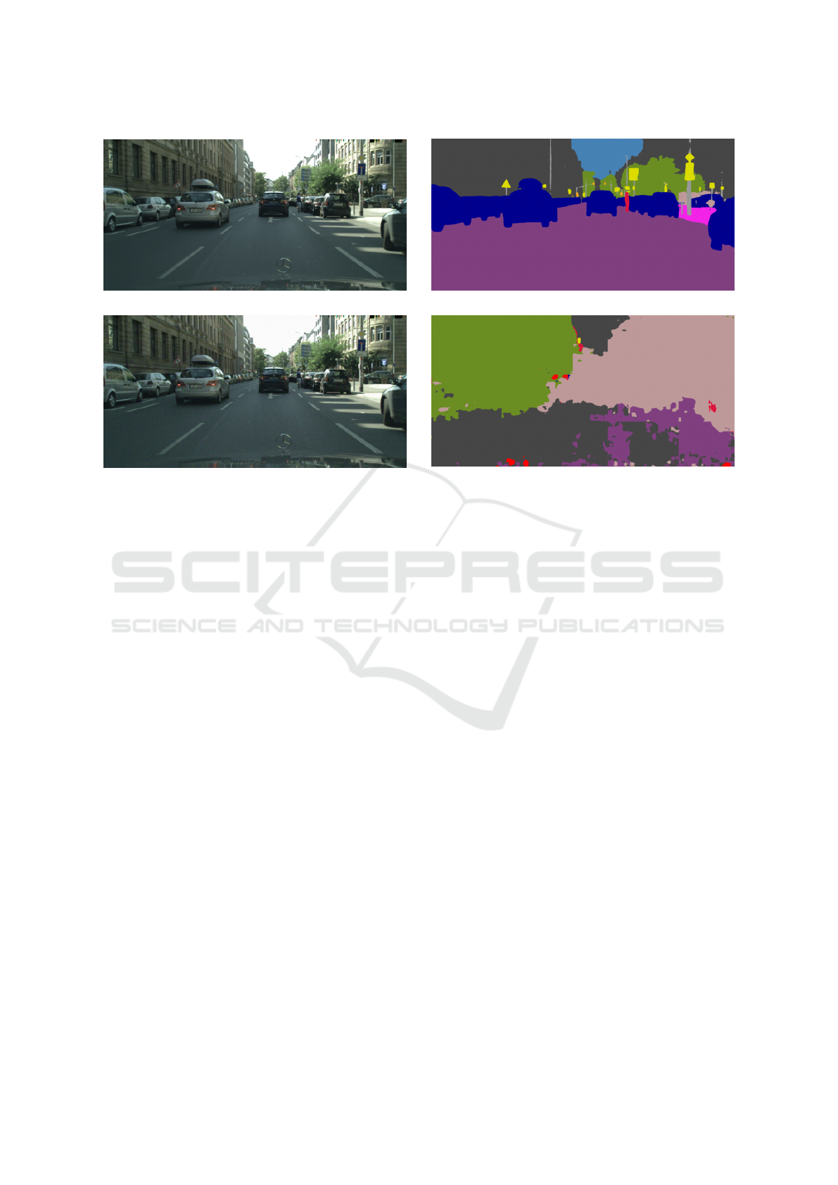
(a) Clean image from Cityscapes (Cordts et al., 2016).

(b) Prediction of the clean image.

Method (ε = 0.03).

(d) Prediction of the adversarial example.

Figure 1: Predictions for a clean input and an adversarial example produced by a deep neural network for semantic segmen-

tation. The two inputs in (a) and (c) look the same for a human observer, but the predictions of the clean image and the

adversarial example shown in (b) and in (d), respectively, are completely different.

through the deep neural network and therefore highly

increases the training time. To reduce the computa-

tional effort of adversarial training Goodfellow et al.

(2015) used the information of just a single gradient

for computing the adversarial examples. But this kind

of single-step adversarial training can be too weak and

it has been observed that overﬁtting can take place,

i.e. the speciﬁc adversarial is classiﬁed correctly, but

not its immediate environment. In particular, it is

not robust against multi-step attacks (Madry et al.,

2018). Recent research discovered that this overﬁt-

ting is caused by using a static step size while creating

the adversarial examples for adversarial training (Kim

et al., 2020). To overcome this, Kim et al. (2020) pro-

pose a method to ﬁnd an ideal step size by evaluating

equidistant points in the direction of the gradient. But

this algorithm is in worst case as expensive as multi-

step adversarial training.

Differently to most of the previous research on

adversarial robustness, we will focus on adversar-

ial training for semantic segmentation in this work.

The task of semantic segmentation is to assign every

pixel of the input image a corresponding class. Be-

cause semantic segmentation needs to address local-

ization and semantic simultaneously, it is a more com-

plicated task than image classiﬁcation (Long et al.,

2015). Consequently, the models for semantic seg-

mentation are generally complex, and therefore the

computational effort to train such models is in prin-

cipal very high. Since adversarial training also neg-

atively affects the training time, our goal is to ﬁnd a

computationally efﬁcient method which at the same

time increases the robustness of semantic segmenta-

tion models effectively.

For this purpose, we extend the idea of robust

single-step adversarial training. On the one hand,

we investigate single-step adversarial training for se-

mantic segmentation as a relevant and challenging ap-

plication problem for deep learning, and we demon-

strate that it shares the problem of overﬁtting and lim-

ited robustness towards multi-step attacks with stan-

dard classiﬁcation problems. On the other hand, we

demonstrate that a careful selection of the step size

can mitigate this problem insofar as even random step

sizes improve robustness. We propose an efﬁcient pa-

rameterless method to choose an optimum step size,

which yields robustness results which are compara-

ble to multi-step adversarial training for two popu-

lar benchmarks from the domain of image segmen-

tation, while sharing the efﬁciency of single-step ap-

proaches.

ICPRAM 2022 - 11th International Conference on Pattern Recognition Applications and Methods

180

2 BACKGROUND AND RELATED

WORK

2.1 Adversarial Training

Adversarial training for a classical image classiﬁ-

cation task tries to solve the following robust op-

timization problem (Shaham et al., 2016): given a

paired sample (x, y) consisting of an input sample

x ∈ X ⊂ [0,1]

H×W×C

and an associated label y ∈ Y ⊂

{1,...,M}, where H, W , C and M are the height, the

width, the number of color channels and the num-

ber of classes, respectively, let ` denote the loss func-

tion of a deep neural network f

: X → [0,1]

, robust

learning aims for the weights θ with

min

(x,y)∈(X,Y )



max

δ∈B(0,ε)

`( f

(x + δ), y)



, (1)

where E and B(0, ε) denote the expected value and

a sphere at origin with radius ε, respectively. The

sphere is dependent on a chosen distance metric. In

the context of adversarial examples most often L

, L

and L

∞

are considered. In this paper we focus only on

∞

Because the loss function is highly nonlinear and

non-convex even solving the inner maximization in

eq. (1) is considered intractable (Katz et al., 2017;

Weng et al., 2018). Therefore, the maximization

problem is often approximated by crafting adversar-

ial examples, such that the optimization of adversarial

training changes to

min

adv

,y)∈(X

adv

,Y )

`( f

adv

),y), (2)

where the adversarial examples x

adv

∈ X

adv

⊂

[0,1]

H×W×C

are generated by a chosen adversarial at-

tack, such that kx − x

adv

∞

≤ ε holds. To guarantee

the classiﬁcation accuracy on the original clean sam-

ples usually x

adv

is randomly set to be a clean sample

or an adversarial example. For crafting adversarial

examples while training, most often gradient based

methods, like the Fast Gradient Sign Method or the

Basic Iterative Method, are used.

2.1.1 Fast Gradient Sign Method

The Fast Gradient Sign Method (FGSM) is a single-

step adversarial attack which is a particularly easy

and computationally cheap gradient based method,

because it uses just a single gradient for calculating

the adversary noise (Goodfellow et al., 2015). If a

step size ε is given, an adversarial example is deter-

mined by

adv

= x + ε · sign(∇

`( f

(x),y)). (3)

Notice, while generating adversarial examples the

color channels of the resulting images can leave their

value range of [0, 1]. To prevent the values of leav-

ing the interval, they are throughout this work always

clipped into the allowed range.

2.1.2 Basic Iterative Method

The Basic Iterative Method (BIM) is a multi-step gen-

eralization of the FGSM (Kurakin et al., 2016). In-

stead of evaluating just one gradient, the BIM uses

n gradients iteratively, to reach a stronger adversarial

example. Given a maximum perturbation ε, a num-

ber of iterations N and a step size α, an adversarial

example created with BIM is given iteratively by

= x,

i+1

= Π

x,ε

+ α · sign (∇

`( f

),y))),

adv

= x

(4)

Where the function ˜p = Π

x,ε

(p) projects p into the

ε-neighbourhood of x, such that k ˜p − xk

∞

≤ ε.

2.2 Restrictions of Single-step

Adversarial Training

To generate adversarial examples while train-

ing, Goodfellow et al. (2015) chose the FGSM as a

computationally cheap adversarial attack. But it was

shown that models trained with such a single-step ad-

versarial training are not robust against multi-step at-

tacks (Madry et al., 2018). Therefore, to train robust

models, multi-step adversarial training is commonly

used. Since multi-step approaches require multiple

forward and backward passes through the deep neural

network, training a robust model becomes computa-

tionally very intensive.

To minimize the computational effort while train-

ing, one line of work tries to increase the robust-

ness of single-step adversarial training. Wong et al.

(2020) analyzed the robustness of single-step adver-

sarial training epoch-wise and observed that the ro-

bustness against BIM increases in the beginning dur-

ing training, but decreases after some epochs. This

observation is called catastrophic overﬁtting. To over-

come this phenomenon Wong et al. (2020) added ran-

dom noise to the input before using the FGSM for

adversarial training and also added early-stopping by

tracking the multi-step robustness of small batches. A

few further approaches follow this line of research (Li

et al., 2020; Andriushchenko and Flammarion, 2020).

Because these methods need to calculate more

than one gradient at some point, they are computa-

tionally inefﬁcient. Kim et al. (2020) showed empiri-

cally that the static step size for generating the adver-

Single-step Adversarial Training for Semantic Segmentation

181

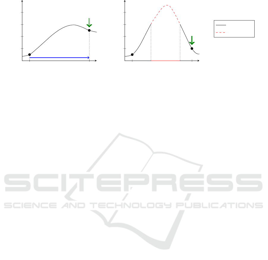
x x

adv

FGSM

static step size

use for

training

direction of gradient

loss

(a) Before catastrophic overﬁtting.

x x

adv

incorrect

prediction

reduced

loss

direction of gradient

loss

(b) Catastrophic overﬁtting.

true class

false class

Figure 2: Sketch: The static step size of single-step adversarial training as reason for catastrophic overﬁtting. (a) After initial

single-step adversarial training the adversarial example is classiﬁed correctly. (b) Further training reduces the loss of the

adversarial example in ﬁxed distance to the original sample even more, but in between the loss increases resulting in a region

of incorrect predictions.

sarial examples constitute a reason why single-step

adversarial training is not robust. Single-step adver-

sarial examples which are generated by a ﬁxed step

size have a ﬁxed distance from their original data

points. When training on such samples as well as on

the original data points, the loss at these points be-

comes very low, but there is no incentive to reduce

the loss between these extremes or to provide a mono-

tonic output in this region. This can lead to catas-

trophic overﬁtting as displayed in ﬁg. 2, i.e. the pre-

diction of the neural network at the original data and

the adversarial examples are correct, but in between

there is a region where the prediction of the network

becomes incorrect. Multi-step adversarial attacks it-

eratively use small step sizes, and therefore are able to

ﬁnd these areas of non-monotonicity, such that single-

step adversarial training is not robust against multi-

step attacks.

To overcome this problem, Kim et al. (2020) pro-

posed to test a range of different step sizes by equidis-

tant sampling in the direction of the gradient and to

choose the smallest step size which leads to an incor-

rect prediction. Since this approach aims for a mini-

mum step size to generate an adversarial sample, we

can expect monotonicity of the network output in be-

tween, at least it is guaranteed that no closer adver-

sarials can be found in the direction of the gradient.

Hence overﬁtting seems less likely in such cases, as

is conﬁrmed by the experimental ﬁnding presented

in (Kim et al., 2020).

Yet, the sampling strategy which is presented

in (Kim et al., 2020) requires several forward passes

through the network and is thus in worst case as de-

manding as multi-step approaches. Additionally, the

strategy is not well suited for semantic segmentation,

because on semantic segmentation it is not deﬁned

whether an adversarial example leads to a false pre-

diction or not. In the following, we propose an ap-

proximate analytic solution how to compute a clos-

est adversarial, which leads to an efﬁcient implemen-

tation of this robust step size selection strategy and

which can be utilized for the task of semantic seg-

mentation.

3 METHODS

3.1 Choosing the Step Size for Image

Classiﬁcation

To explain the idea behind our step size control al-

gorithm, we ﬁrst start looking at image classiﬁca-

tion. We are interested in an efﬁcient analytic approx-

imation which yields in the direction of the gradient

the closest adversarial example, i.e. a closest pattern

where the classiﬁcation changes.

The deep neural network is given as a function

: X → [0, 1]

, where the output of the deep neural

network f

(x) is computed using the softmax func-

tion. The inputs to the softmax z(x) are called logits.

We deﬁne the gain function g : X ×Y → R as

g(x, y) = z

(x) − max

i6=y

(x), (5)

where z

(x) is the logit value of class i. The gain func-

tion in eq. (5) has the property that

g(x, y)



> 0 if argmax f

(x) = y

≤ 0 else

. (6)

For given (x,y) a close adversarial example can be

found at the decision boundary between a correct and

ICPRAM 2022 - 11th International Conference on Pattern Recognition Applications and Methods

182

an incorrect prediction, which holds if

g(x

adv

,y) = 0. (7)

Using the update rule of the FGSM in eq. (3) on the

gain function, we create an adversarial example by

adv

= x − ε · sign(∇

g(x, y)). (8)

For estimating the step size ε, we linearly approxi-

mate the gain function g with a Taylor approximation

g(x

adv

,y) ≈ g(x, y) + (x

adv

− x)

· ∇

g(x, y). (9)

Combining eq. (7), eq. (8) and eq. (9) results in

0 = g(x, y) − ε · sign(∇

g(x, y))

· ∇

g(x, y), (10)

which we can solve for the step size ε:

ε =

g(x, y)

∇

g(x, y)

· sign(∇

g(x, y))

g(x, y)

k∇

g(x, y)k

(11)

Notice, the idea of the above step size control is the

same as doing one step of Newton’s approximation

method for ﬁnding the zero crossings of a function.

We therefore call our approach Fast Newton Method.

Contrary to the classical solution of robust opti-

mization, we use an approximation of the closest ad-

versarial example for training. This has two effects:

on the one hand, we expect monotonicity of the pre-

diction in between, or a sufﬁcient distance from 0.

Hence a network which classiﬁes x and the closest ad-

versarial correctly likely classiﬁes the enclosed inter-

val in the same way, avoiding catastrophic overﬁtting.

On the other hand, we do not consider any predeﬁned

radius; rather we use the smallest radius that includes

an adversarial example. Using these adversarial ex-

amples for training, iteratively increases the radius of

the sphere, and consequently the distance where ad-

versarials can be found.

3.2 Robust Semantic Segmentation

The above mentioned results were presented in the

context of image classiﬁcation. In this work we want

to concentrate on semantic segmentation. It is al-

ready known that deep neural networks for seman-

tic segmentation are also vulnerable against adversar-

ial examples (Xie et al., 2017; Metzen et al., 2017),

but only few approaches address the question how to

efﬁciently implement robust training for image seg-

mentation tasks. As far as we know, there is only

one work investigating the impact of multi-step ad-

versarial training on semantic segmentation (Xu et al.,

2020).

First, we formalize the learning objective for ro-

bust semantic segmentation. Because semantic seg-

mentation determines the class of each single pixel

of an image, semantic segmentation could be inter-

preted as multiple pixel-wise classiﬁcations. To pre-

dict all the pixels at the same time the deep neu-

ral network function f

: X → [0, 1]

H×W×M

has in-

creased output dimension. The set of labels are given

by Y ⊂ {1, . . .,M}

H×W

. Robust learning on semantic

segmentation tries to optimize

min

(x,y)∈(X,Y )



max

δ∈B(0,ε)

∑

j=0

`( f

θ, j

(x + δ),y

)



(12)

for the weights θ, where f

θ, j

(x) and y

are the predic-

tion and the label of the j-th pixel, respectively. To

ﬁnd the weights for all the pixel-wise predictions si-

multaneously, the losses of the pixel-wise predictions

are averaged.

Adversarial training on semantic image segmenta-

tion approximates the min-max loss by the following

term:

min

adv

,y)∈(X

adv

,Y )

∑

j=0

`( f

θ, j

adv

),y

), (13)

where x

adv

∈ X

adv

constitutes a suitable image with

kx−x

adv

∞

≤ ε, which plays the role of an adversarial

in the sense that it leads to an error of the segmented

image for a large number of pixels. Yet, unlike for

scalar outputs, it is not clear what exactly should be

referred to by an adversarial: we can aim for an in-

put x

adv

such that all output pixels change, or, alter-

natively, approximate this computationally extensive

extreme by an efﬁcient surrogate, as we will introduce

in the following.

3.3 Choosing the Step Size for Semantic

Segmentation

Initially, we treat each pixel as a separate output. An

adversarial corresponds to an input such that one spe-

ciﬁc output pixel changes. For this setting, the gain

function from eq. (5) becomes:

(x, y

) = z

j,y

(x) − max

i6=y

j,i

(x), (14)

for j ∈ {1, . . .,HW }, where z

j,i

(x) is the logit value

of the j-th pixel of class i. To ﬁnd a close adversar-

ial example x

adv

which changes all (or a large num-

ber of) pixels, each pixel-wise output should be at the

boundary between a correct and an incorrect predic-

tion. This holds if

adv

) = 0, ∀ j ∈ {1, . ..,HW }. (15)

Single-step Adversarial Training for Semantic Segmentation

183

Using our results from sec. 3.1, we obtain a differ-

ent step size ε

for every pixel, hence a possibly dif-

ferent adversarial x

( j)

adv

for each pixel-wise prediction.

A common adversarial example x

adv

which approxi-

mately suits for all pixel-wise predictions in the same

time, could be chosen as the average term

adv

∑

j=1

( j)

adv

. (16)

But this procedure requires the computation of HW

different gradients ∇

(x, y

) for j = 1, . ..,HW

which is computational too expensive to work with.

As an alternative, we can refer to adversarial

examples as images for which a number of pixels

change the segmentation assignment. In this case

we consider the pixel-wise predictions at the same

time from the beginning by using the average of the

gain functions (rather than the average of the speciﬁc

pixel-wise adversarials). A close adversarial example

in this sense is then given if

∑

j=1

adv

) = 0. (17)

Deﬁning the averaged gain function as ¯g(x, y) =

∑

j=1

(x, y

) and using our method from sec. 3.1

results in a single step size

ε =

¯g(x, y)

k∇

¯g(x, y)k

, (18)

such that the update rule for ﬁnding an adversarial ex-

ample becomes

adv

= x −

¯g(x, y)

k∇

¯g(x, y)k

· sign(∇

¯g(x, y)). (19)

Of course using the averaged gain function for calcu-

lating the step size ε in eq. (18) leads to a more loose

approximation, but as a trade off this method does not

increase the computational effort compared to adver-

sarial training with the FGSM considerably, because

we also calculate just one gradient.

4 EXPERIMENTS

4.1 Implementation

4.1.1 Datasets

To evaluate our approach, we use the datasets

Cityscapes (Cordts et al., 2016) and PASCAL

VOC (Everingham et al., 2015). Cityscapes con-

tains 2975, 500 and 1525 colored images of size

1024 × 2048 for training, validation and testing, re-

spectively. The labels assign most pixels one of 19

classes, where some areas are not labeled.

PASCAL VOC originally includes 1464, 1499 and

1456 differently sized images for training, validation

and testing, respectively. Later the training set was

increased to 10582 images (Hariharan et al., 2011).

Including the background class, the pixels are labeled

as one of 21 classes. Like in Cityscapes there are also

some areas not labeled, such that we limit our loss and

gain function for both datasets to the labeled pixels.

We always normalise the color channels in the range

of [0,1].

4.1.2 Model

As base model we chose the popular PSPNet50 archi-

tecture from (Zhao et al., 2017) with a slight modiﬁ-

cation. Instead of using ResNet50 we work with the

improved ResNet50v2 as fundamental pretrained net-

work (He et al., 2016). For the training parameters

we follow the paper (Zhao et al., 2017) using SGD

with a momentum of 0.9. The learning rate decays

polynomially with a base learn rate of 0.01 and power

0.9. We use a batchsize of 16 and also include L

weight decay of 10

−4

. However, for a better compari-

son to different models, we do not apply the auxiliary

loss from (Zhao et al., 2017). To further increase the

variation of the dataset, the data is randomly horizon-

tally ﬂipped, resized between 0.5 and 2, rotated be-

tween −10 and 10 degrees, and additionally randomly

blurred. Afterwards, we randomly crop the images to

a size of 712 × 712 and 472 × 472 for Cityscapes and

PASCAL VOC, respectively. For evaluation, we will

compare the robustness of the following models:

• The Basic Model without using any adversarial

examples in training,

• The FGSM Model trained with FGSM at ε = 0.03,

• The random FGSM Model trained with FGSM at

ε ∼ U(0,0.03) chosen uniformly,

• The BIM Model trained with BIM (α = 0.01, ε =

0.03, N = 3),

• Fast Newton Method trained with our algorithm,

where the parameters of the BIM Model are taken

from (Xu et al., 2020). For adversarial training the

input is randomly chosen either a clean data sample

or an adversarial example, each with probability of

0.5.

4.1.3 Evaluating the Robustness

We measure the performance on the clean and

the adversary data with the mean Intersection over

ICPRAM 2022 - 11th International Conference on Pattern Recognition Applications and Methods

184

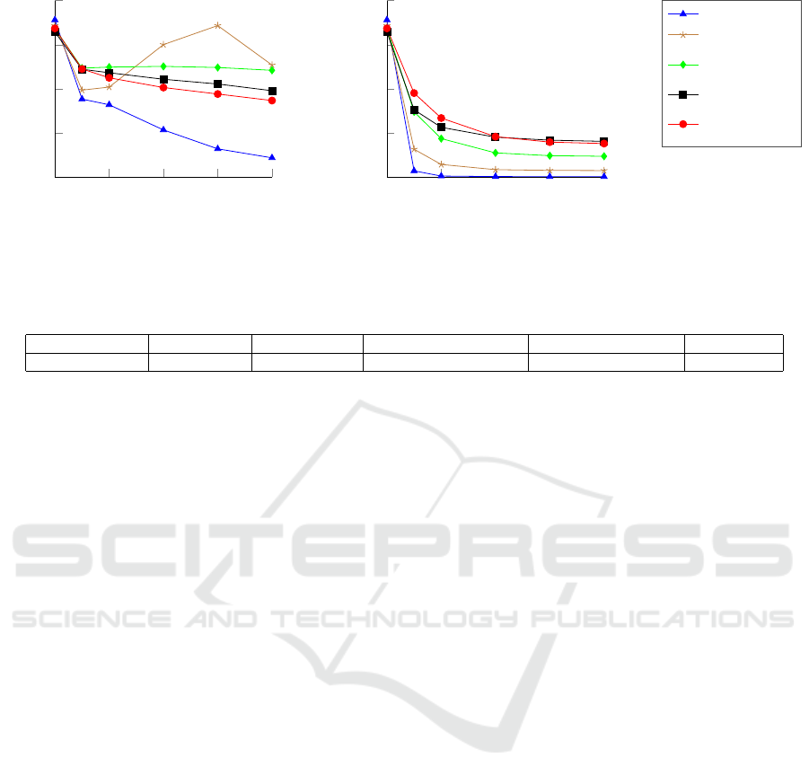
0 0.01 0.02 0.03 0.04

0.2

0.4

0.6

0.8

mean IoU

(a) Robustness against single-step adversarial

examples created with FGSM.

0 0.01 0.02 0.03 0.04

0.2

0.4

0.6

0.8

mean IoU

(b) Robustness against adversarial examples

created with BIM (N = 10, α = 0.004).

Basic Model

FGSM Model

random

FSGM Model

BIM Model

Fast Newton

Method

Figure 3: Robustness curves on the Cityscapes dataset.

Table 1: Additional training time on Cityscapes shown as percentage compared to the training time of the Basic Model.

Method Basic Model FGSM Model random FGSM Model Fast Newton Method BIM Model

Additional time 0.00% 12.52% 12.34% 11.98% 45.92%

Unit (IoU) (Everingham et al., 2015). The mean IoU

is a standard measure for semantic segmentation. It is

used over the standard accuracy per Pixel, because it

better represents the desired accuracy in case of dif-

ferently sized objects.

For the empirical robustness evaluation we at-

tack each model with FGSM and BIM. The adversar-

ial examples are generated by maximizing the cross-

entropy loss. For both attacks we vary the attack ra-

dius ε from 0 to 0.04, such that we receive one ro-

bustness curve for each model and attack. As trade

off between computational time and attack strength,

we use BIM with N = 10 iterations. We chose the

step size α as small as possible, such that the maxi-

mum perturbation rate of ε = 0.04 is still reachable.

Hence, we use α = 0.004 as step size for BIM.

4.2 Results on Cityscapes

4.2.1 Single-step Robustness

In ﬁg. 3(a) are the summarized results regarding the

FGSM shown. We see that the mean IoU of all mod-

els except the FGSM Model and the random FGSM

Model decrease with increased attack strength ε,

whereas the performance of the BIM Model and our

Fast Newton Method decrease slower. The BIM

Model shows slightly better robustness than ours, but

the FGSM Model and the random FGSM Model per-

form even better. Looking closer to the robustness

curve of the FGSM Model, we observe that the model

is most robust to adversarial examples with attack

strength ε = 0 and ε = 0.03. For the other val-

ues of ε the robustness decreases. This observation

matches with the phenomenon of catastrophic over-

ﬁtting shown in ﬁg. 2. The model is most robust ex-

actly against the adversarial examples it was trained

for. For the values between ε = 0 and ε = 0.03 the

nonlinear character of deep neural networks leads to

a drop in the robustness.

4.2.2 Multi-step Robustness

Fig. 3(b) shows the robustness of the trained models

against attacks with BIM. As can be seen, all models

perform signiﬁcantly worse against this attack. Be-

cause the robustness is deﬁned as the performance

under the worst case attack, this evaluation represents

the real robustness of the models far better. We can

see that the Basic Model and FGSM Model drop very

fast with increased attack strength ε. So we can con-

ﬁrm that the FGSM Model overﬁts. Even though the

Fast Newton Method and the random FGSM Model

are also single-step adversarial training models, they

perform signiﬁcantly better under the attack with BIM

than the FGSM Model. That shows that the idea of

controlling the step sizes of adversarial attacks makes

single-step adversarial training more effective. The

performance of our Fast Newton Method compared

to the FGSM models shows the importance of choos-

ing the correct step size for creating adversarial exam-

ples during training. Additionally, our Fast Newton

Method shows for small ε even better robustness than

the more sophisticated BIM model, and is for larger ε

equally robust while being signiﬁcantly less compu-

tational expensive (see table 1).

Single-step Adversarial Training for Semantic Segmentation

185

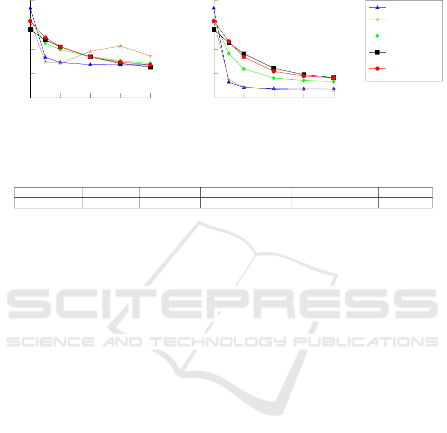
0 0.01 0.02 0.03 0.04

0.2

0.4

0.6

0.8

mean IoU

(a) Robustness against adversarial examples

created with FGSM.

0 0.01 0.02 0.03 0.04

0.2

0.4

0.6

0.8

mean IoU

(b) Robustness against adversarial examples

created with BIM (N = 10, α = 0.004).

Basic Model

FGSM Model

random

FSGM Model

BIM Model

Fast Newton

Method

Figure 4: Robustness curves on the PASCAL VOC dataset.

Table 2: Additional training time on PASCAL VOC shown as percentage compared to the training time of the Basic Model.

Method Basic Model FGSM Model random FGSM Model Fast Newton Method BIM Model

Additional time 0.00% 31.76% 34.71% 31.18% 98.24%

4.3 Results on PASCAL VOC

4.3.1 Single-step Robustness

The robustness curves against the FGSM for models

trained on PASCAL VOC are shown in ﬁg. 4(a). We

observe that the attack is not as effective on the Basic

Model as on Cityscapes. We think that this is mainly

reasoned in the characteristic of the dataset with its

dominant background class. It seems difﬁcult for the

attack to switch the class of the whole background

area. But as we already mentioned, the robustness is

better represented by a strong multi-step attack. Our

focus here lays again in the curve course of the FGSM

Model. Like on Cityscapes the FGSM Model is most

robust against the adversarial examples it was trained

for (ε = 0 and ε = 0.03). So we see again an indicator

for catastrophic overﬁtting.

4.3.2 Multi-step Robustness

Looking in Fig. 4(b) on the robustness of the trained

models against the BIM, we can observe very sim-

ilar results like on Cityscapes. Both, the Basic and

the FGSM Model, perform much worse than the other

models. So we can clearly say that the FGSM Model

overﬁts to adversarial examples it was trained with.

However, even if the random FGSM Model and the

Fast Newton Method are trained with single-step ad-

versarial examples, too, they perform signiﬁcantly

better than the FGSM Model. Thus, we can conﬁrm

that varying the step size increases the robustness of

such models. Because the Fast Newton Method out-

performs the random FGSM Model, we conclude that

our proposed step size is more superior than determin-

ing the step size randomly. Additionally, even if our

Fast Newton Method is less computational expensive

than the BIM Model (see table 2), their robustness is

very similar.

5 CONCLUSION

The research community focused so far on improv-

ing the robustness of deep neural networks for im-

age classiﬁcation. We on the other hand concentrate

on semantic segmentation. We showed that single-

step adversarial training for semantic segmentation

underlies the same difﬁculties regarding the robust-

ness against multi-step adversarial attacks. One rea-

son for that non-robustness of single step adversarial

training is the static step size for ﬁnding the adver-

sarial examples while training. Therefore, we pre-

sented a step size control algorithm which approxi-

mates an appropriate step size for every input such

that the robustness of single-step adversarial training

increases signiﬁcantly. As our method approximates

the best step size based on the gradient, which needs

to be calculated anyway for adversarial training, our

method does not considerably increase the computa-

tional effort while training a signiﬁcantly more robust

model. In addition, our approach is easy to use, be-

cause it is free of any parameter. Finally, we showed

on the datasets Cityscapes and PASCAL VOC, that

our method equals in performance with the more so-

phisticated and the more computationally expensive

multi-step adversarial training.

ICPRAM 2022 - 11th International Conference on Pattern Recognition Applications and Methods

186

REFERENCES

Andriushchenko, M. and Flammarion, N. (2020). Under-

standing and improving fast adversarial training. In

Advances in Neural Information Processing Systems.

Curran Associates, Inc.

Cohen, J., Rosenfeld, E., and Kolter, Z. (2019). Certiﬁed

adversarial robustness via randomized smoothing. In

36th International Conference on Machine Learning.

PMLR.

Cordts, M., Omran, M., Ramos, S., Refeld, T., Enzweiler,

M., Benenson, R., Franke, U., Roth, S., and Schielde,

B. (2016). The cityscapes dataset for semantic urban

scene understanding. In IEEE Conference on Com-

puter Vision and Pattern Recognition (CVPR).

Everingham, M., Eslami, S., Gool, L. V., Williams, C.,

Winn, J., and Zisserman, A. (2015). The pascal vi-

sual object classes challenge: A retrospective. In Int J

Comput Vis.

Goodfellow, I., Shlens, J., and Szegedy, C. (2015). Explain-

ing and harnessing adversarial examples. In 3rd In-

ternational Conference on Learning Representations,

ICLR 2015.

Hariharan, B., Arbelaez, P., Bourdev, L., Maji, S., and Ma-

lik, J. (2011). Semantic contours from inverse detec-

tors. In International Conference on Computer Vision

(ICCV).

He, K., Zhang, X., Ren, S., and Sun, J. (2016). Identity

mappings in deep residual networks. In Computer Vi-

sion – ECCV 2016. Springer International Publishing.

Katz, G., Barrett, C., Dill, D., Julian, K., and Kochender-

fer, M. (2017). Reluplex: An efﬁcient smt solver for

verifying deep neural networks. In Computer Aided

Veriﬁcation. Springer International Publishing.

Kim, H., Lee, W., and Lee, J. (2020). Understanding catas-

trophic overﬁtting in single-step adversarial training.

arXiv. Last accessed 20 April 2021.

Kurakin, A., Goodfelow, I., and Bengio, S. (2016). Adver-

sarial examples in the physical world. CoRR.

Li, B., Wang, S., Jana, S., and Carin, L. (2020). Towards

understanding fast adversarial training. arXiv. Last

accessed 20 April 2021.

Long, J., Shelhamer, E., and Darrell, T. (2015). Fully con-

volutional networks for semantic segmentation. In

IEEE Conference on Computer Vision and Pattern

Recognition (CVPR).

Madry, A., Makelov, A., Schmidt, L., Tsipras, D., and

Vladu, A. (2018). Towards deep learning models

resistant to adversarial attacks. In 6th International

Conference on Learning Representations, ICLR 2018.

Metzen, J., Kumar, M., Brox, T., and Fischer, V. (2017).

Universal adversarial perturbations against semantic

image segmentation. In IEEE International Confer-

ence on Computer Vision (ICCV).

Raghunathan, A., Steinhardt, J., and Liang, P. (2018). Cer-

tiﬁed defenses against adversarial examples. In 6th In-

ternational Conference on Learning Representations,

ICLR 2018.

Shaham, U., Yamada, Y., and Negahban, S. (2016). Under-

standing adversarial training: Increasing local stabil-

ity of neural nets through robust optimization. Neuro-

computing.

Stutz, D., Hein, M., and Schiele, B. (2020). Conﬁdence-

calibrated adversarial training: Generalizing to unseen

attacks. In 37th International Conference on Machine

Learning. PMLR.

Szegedy, C., Zaremba, W., Sutskever, I., Bruna, J., Erhan,

D., Goodfellow, I., and Fergus, R. (2014). Intriguing

properties of neural networks. In 2nd International

Conference on Learning Representations, ICLR 2014.

Weng, T., Zhang, H., Chen, H., Song, Z., Hsieh, C., Bon-

ing, D., Dhillon, I., and Daniel, L. (2018). Towards

fast computation of certiﬁed robustness for ReLU net-

works. In 35th International Conference on Machine

Learning. PMLR.

Willers, O., Sudholt, S., Raafatnia, S., and Abrecht, S.

(2020). Safety concerns and mitigation approaches

regarding the use of deep learning in safety-critical

perception tasks. In Computer Safety, Reliability, and

Security. SAFECOMP 2020 Workshops. Springer In-

ternational Publishing.

Wong, E. and Kolter, Z. (2018). Provable defenses against

adversarial examples via the convex outer adversarial

polytope. In 35th International Conference on Ma-

chine Learning. PMLR.

Wong, E., Rice, L., and Kolter, Z. (2020). Fast is better

than free: Revisiting adversarial training. In 8th In-

ternational Conference on Learning Representations,

ICLR 2020.

Xie, C., Wang, J., Zhang, Z., Zhou, Y., Xie, L., and Yuille,

A. (2017). Adversarial examples for semantic seg-

mentation and object detection. In IEEE International

Conference on Computer Vision (ICCV).

Xu, X., Zhao, H., and Jia, J. (2020). Dynamic divide-and-

conquer adversarial training for robust semantic seg-

mentation. arXiv. Last accessed 20 April 2021.

Zhao, H., Shi, J., Qi, X., Wang, X., and Jia, J. (2017). Pyra-

mid scene parsing network. In IEEE Conference on

Computer Vision and Pattern Recognition (CVPR).

Single-step Adversarial Training for Semantic Segmentation

187