A k-Means Algorithm for Clustering with Soft Must-link and

Cannot-link Constraints

Philipp Baumann

1 a

and Dorit S. Hochbaum

2 b

Department of Business Administration, University of Bern, Schuetzenmattstrasse 14, 3012 Bern, Switzerland

IEOR Department, University of California, Berkeley, Etcheverry Hall, CA 94720, U.S.A.

Keywords:

Constrained Clustering, Must-link and Cannot-link Constraints, Mixed-binary Linear Programming.

Abstract:

The k-means algorithm is one of the most widely-used algorithms in clustering. It is known to be effective

when the clusters are homogeneous and well separated in the feature space. When this is not the case, incor-

porating pairwise must-link and cannot-link constraints can improve the quality of the resulting clusters. Var-

ious extensions of the k-means algorithm have been proposed that incorporate the must-link and cannot-link

constraints using heuristics. We introduce a different approach that uses a new mixed-integer programming

formulation. In our approach, the pairwise constraints are incorporated as soft-constraints that can be violated

subject to a penalty. In a computational study based on 25 data sets, we compare the proposed algorithm to a

state-of-the-art algorithm that was previously shown to dominate the other algorithms in this area. The results

demonstrate that the proposed algorithm provides better clusterings and requires considerably less running

time than the state-of-the-art algorithm. Moreover, we found that the ability to vary the penalty is beneﬁcial in

situations where the pairwise constraints are noisy due to corrupt ground truth.

1 INTRODUCTION

In many practical clustering applications, users have

some side information about the clustering solution.

For example, users might know the labels of a small

set of objects. Using this side information to guide

the clustering algorithms can greatly improve clus-

tering quality, especially when clusters have irregu-

lar shapes and are not well separated in the feature

space. A common approach to incorporate side infor-

mation is to specify must-link (ML) and cannot-link

(CL) constraints for pairs of objects. An ML con-

straint states that two objects belong to the same clus-

ter while a CL constraint states that two objects be-

long to different clusters. Successful applications of

clustering with ML and CL constraints include lane

ﬁnding in GPS data (Wagstaff et al., 2001), text cat-

egorization (Basu et al., 2004), image and video seg-

mentation (Wu et al., 2013), and clustering of time

series (Lampert et al., 2018).

We consider here a constrained clustering problem

where a set of objects must be assigned to a predeﬁned

number of clusters. The ML and CL constraints can

https://orcid.org/0000-0002-3286-4474

https://orcid.org/0000-0002-2498-0512

be used as guidance rather than hard requirements,

i.e., not all ML and CL constraints must be enforced.

Various algorithms have been developed for clus-

tering with ML and CL constraints. Many of

them are adaptations of traditional clustering algo-

rithms. Adaptations of the k-means algorithm include

the constrained k-means algorithm (COP-kmeans) of

(Wagstaff et al., 2001), the pairwise constrained clus-

tering algorithm (PCK-means) of (Basu et al., 2004),

the constrained vector quantization error algorithm

(CVQE) of (Davidson and Ravi, 2005), the linear

version of the CVQE algorithm (LCVQE) proposed

by (Pelleg and Baras, 2007), and the lagrangian con-

strained clustering algorithm (LCC) of (Ganji et al.,

2016). (Gonz

alez-Almagro et al., 2020) recently con-

ducted a comprehensive computational comparison of

seven algorithms that included the COP-kmeans and

the LCVQE algorithms. It turned out that the dual

iterative local search algorithm (DILS) of (Gonz

alez-

Almagro et al., 2020) is the currently leading algo-

rithm in terms of clustering quality. A shared charac-

teristic of established algorithms for clustering with

ML and CL constraints is that they all use heuristics

to incorporate the ML and CL constraints.

We propose here an alternative approach to incor-

porate ML and CL constraints that is based on mixed-

Baumann, P. and Hochbaum, D.

A k-Means Algorithm for Clustering with Soft Must-link and Cannot-link Constraints.

DOI: 10.5220/0010800000003122

In Proceedings of the 11th International Conference on Pattern Recognition Applications and Methods (ICPRAM 2022), pages 195-202

ISBN: 978-989-758-549-4; ISSN: 2184-4313

195

integer programming. Our algorithm, which we refer

to as BH-kmeans, is an adaptation of the k-means al-

gorithm that assigns, in each iteration, all objects to

clusters by solving a mixed-binary linear optimization

program. The ML and CL constraints are included in

the program as soft constraints. In contrast to most

other algorithms that treat the ML and CL constraints

as soft constraints, our algorithm provides a parame-

ter to control the penalty that is incurred for violating

a constraint. This allows to adjust the algorithm to

different levels of noise in the constraint set.

In a computational analysis based on 100 problem

instances from the literature, we compare our BH-

kmeans algorithm to the DILS algorithm (Gonz

alez-

Almagro et al., 2020). Our results indicate that the

BH-kmeans algorithm clearly outperforms the DILS

algorithm in clustering quality and running time.

Furthermore, we analyze, based on constraint sets

that differ with respect to the amount of noise, how

changes of the penalty parameter affect the perfor-

mance and the running time of the BH-kmeans al-

gorithm. To the best of our knowledge, this is the

ﬁrst paper that systematically investigates this rela-

tionship.

The paper is structured as follows. In Section 2,

we deﬁne the constrained clustering problem that we

consider here. In Section 3, we describe the BH-

kmeans algorithm. In Section 4, we compare the BH-

kmeans algorithm to the DILS algorithm using prob-

lem instances from the literature. In Section 5, we

analyze the impact of the penalty of soft constraints

on the clustering quality and the running time of the

BH-kmeans algorithm. Finally, in Section 6, we pro-

vide conclusions and directions for future research.

2 CONSTRAINED CLUSTERING

PROBLEM

Given is a data set with n objects, represented by vec-

tors v

, . . . , v

∈ R

of d numeric features. The goal is

to assign a label l

∈ {1, . . . , k} to each object such that

the data set is partitioned into k clusters. The ML and

the CL constraints are deﬁned for pairs of objects. An

ML constraint suggests that two objects i and i

have

the same label. A CL constraint suggests that two ob-

jects i and i

have different labels. The ML and CL

constraints can be used for guidance but they are not

hard requirements that need to be satisﬁed.

The clustering quality can be assessed with inter-

nal or external evaluation measures. Internal evalua-

tion measures are computed based on the same data

that was used for clustering. These measures assume

that objects in the same cluster are more similar than

objects in different clusters according to some similar-

ity measure. External evaluation measures are com-

puted based on external data (e.g., a ground truth as-

signment) that was not used for clustering. In Sec-

tion 4.3, we describe the measures we use in our com-

putational experiments.

3 BH-KMEANS ALGORITHM

Our algorithm ﬁrst determines the initial position ¯c

for each cluster center j = 1, . . . , k by applying the

k-means++ procedure of (Arthur and Vassilvitskii,

2007). This procedure tends to ﬁnd initial positions

that are far away from each other. The algorithm then

alternates between an object assignment and a cluster

center update step until a stopping criterion is met.

1. In the assignment step, the mixed-binary linear

program P (given below) is solved to assign the

objects to the cluster centers. Table 1 contains a

description of the notation.











Min.

∑

i=1

∑

j=1

i j

+M p(

∑

(i,i

)∈CL

∑

(i,i

)∈ML

) (1)

s.t.

∑

j=1

i j

= 1 (i = 1, . . . , n) (2)

∑

i=1

i j

≥ 1 ( j = 1, . . . , k) (3)

i j

+ x

≤ 1 + y

((i, i

) ∈ CL; j = 1, . . . , k) (4)

i j

− x

≤ z

((i, i

) ∈ ML; j = 1, . . . , k) (5)

i j

∈ {0, 1}

(i = 1, . . . , n; j = 1, . . . , k) (6)

≥ 0 ((i, i

) ∈ CL) (7)

≥ 0 ((i, i

) ∈ ML) (8)

The objective function consists of two terms. The

ﬁrst term computes the total Euclidean distance

between the objects and the centers of the clusters

to which they are assigned to. The second term

computes the total penalty that results from vio-

lating ML and CL constraints. Each violation of

an ML or CL constraint contributes Mp to the ob-

jective function, where parameter M is the maxi-

ICPRAM 2022 - 11th International Conference on Pattern Recognition Applications and Methods

196

Table 1: Notation.

Sets

ML Must-link pairs

CL Cannot-link pairs

Parameters

n Number of objects

k Number of clusters

¯c

Center of cluster j

i j

Euclidean distance between object v

and

center ¯c

M Maximum distance (max

i=1,...,n; j=1...,k

i j

)

p Control parameter for penalty

Decision variables

i j

=1, if object i is assigned to cluster j; =0,

else

Auxiliary variables that capture violations

of CL constraints

Auxiliary variables that capture violations

of ML constraints

mum distance between any object i and any clus-

ter center j and parameter p is user-deﬁned. Note

that M must be recomputed in each assignment

step, because the positions of the cluster centers

change in the update step. Constraints (2) ensure

that each object is assigned to exactly one cluster.

Constraints (3) guarantee that each cluster con-

tains at least one object. Constraints (4) incorpo-

rate the CL constraints. The auxiliary variable y

must be set to one if objects i and i

are assigned to

the same cluster j. Constraints (5) incorporate the

ML constraints. The auxiliary variable z

must

be set to one if objects i and i

are assigned to

different clusters. Constraints (6)–(8) deﬁne the

domains of the decision variables.

2. In the update step, the positions of the cluster

centers are recomputed as follows. With C

being

the set of objects assigned to cluster j, the new

cluster center is then computed as ¯c

∑

i∈C

Let OFV

be the objective function after t update

steps. The algorithm alternates between the assign-

ment and update step until either a predeﬁned time

limit has been reached or if OFV

t−1

− OFV

is non-

positive. We implemented these stopping criteria be-

cause we have no proof that the algorithm is guaran-

teed to converge. Since the k-means++ procedure is a

randomized procedure, we obtain different solutions

when we apply the BH-kmeans algorithm with differ-

ent random seeds. A version of the BH-kmeans al-

gorithm that treats all ML and CL constraints as hard

constraints is presented in (Baumann, 2020).

4 COMPUTATIONAL ANALYSIS

WITH NOISE-FREE

CONSTRAINTS

In this section, we experimentally compare the per-

formance of the BH-kmeans algorithm to the perfor-

mance of the DILS algorithm. In Section 4.1, we

describe the problem instances. In Section 4.2, we

brieﬂy describe the DILS algorithm. In Section 4.3,

we explain the performance measures that we use to

evaluate the algorithms. Finally, in Section 4.4, we

explain the experimental design and report the numer-

ical results.

4.1 Problem Instances

We use the 25 data sets from (Gonz

alez-Almagro

et al., 2020). This collection includes data sets which

have non-convex clusters that the standard (uncon-

strained) k-means algorithm fails to discover. We did

not perform any preprocessing of these data sets with

one exception. In the data set Saheart, we replaced

the two non-numeric categories Present and Absent

of the binary feature “Famhist” with one and zero, re-

spectively. (Gonz

alez-Almagro et al., 2020) gener-

ated four different constraint sets for each of the 25

data sets. The four constraint sets are associated with

the four percentages 5%, 10%, 15%, and 20% and are

thus named CS5, CS10, CS15, and CS20. The num-

ber of constraints in the constraint sets is

−1)

with n

= dn × f e, where n is the number of objects in

the data set and f the percentage associated with the

constraint set. Note that all constraints in these con-

straint sets are sampled from the ground truth, i.e.,

they are noise free. We noticed however, that the

constraint sets for the data sets Iris and Wine con-

tain ML and CL constraints that do not comply with

the ground truth. For these two data sets, we gen-

erated our own constraint sets according to the pro-

cedure described in (Gonz

alez-Almagro et al., 2020).

The newly generated constraint sets are available on

github

. The data sets and the other constraint sets

can be downloaded by using the links provided in

(Gonz

alez-Almagro et al., 2020). Since there are four

constraint sets for each data set, the test set comprises

100 problem instances.

4.2 Benchmark Algorithm

We use as benchmark the DILS algorithm of

(Gonz

alez-Almagro et al., 2020). The DILS algo-

rithm is a metaheuristic that keeps only two indi-

https://github.com/phil85/BH-kmeans

A k-Means Algorithm for Clustering with Soft Must-link and Cannot-link Constraints

197

viduals in memory at all times. Mutation and re-

combination operations are applied to the two indi-

viduals to escape from local optima. After applying

the mutation and recombination operations, an iter-

ative local search procedure is used to improve the

two individuals. The DILS algorithm outperformed

six established algorithms for clustering with ML and

CL constraints in a recent computational comparison

(Gonz

alez-Almagro et al., 2020). The comparison in-

cluded the COP-kmeans algorithm and the LCVQE

algorithm that we mention in the introduction, the

two views clustering algorithm (TVClust) and the

relation dirichlet process algorithm (RDP-means) of

(Khashabi et al., 2015), the biased random-key ge-

netic algorithm with local search (BRKGA + LS) of

(de Oliveira et al., 2017), and the constrained eviden-

tial c-means algorithm (CECM) of (Antoine et al.,

2012). Since the DILS algorithm outperformed the

other algorithms, we do not include the other algo-

rithms in our comparison.

4.3 Performance Measures

We use the following four measures to assess the per-

formance of the algorithms. First, we compute the

Adjusted Rand Index (ARI) to assess the ability of

the algorithms to discover a ground truth assignment.

This ability is important if the algorithms are em-

ployed as semi-supervised algorithms for classiﬁca-

tion tasks. In most data sets used here, the ground

truth assignment does not form well-separated clus-

ters of convex shape. Hence, to discover the ground

truth assignment it is necessary to consider the ML

and CL constraints. The ARI takes as inputs the true

labels and the labels assigned by the clustering algo-

rithm and outputs a value in the interval [-1, 1]. A

value close to 1 indicates a high agreement between

the respective partitions and a value close to 0 indi-

cates a low agreement. A value below zero indicates

that the agreement is smaller than the expected agree-

ment that would result when comparing the true parti-

tion to a random partition. Second, we use the within-

cluster sum-of-squares criterion (WCSS) to assess the

ability of the algorithms to detect homogeneous clus-

ters. This criterion corresponds to the sum of the

squared Euclidean distances between objects and the

centroid (mean) of the cluster they are assigned to.

Third, we determine the total number of constraint

violations to assess the ability of the algorithm to sat-

isfy the ML and CL constraints. Fourth, we record

the running time to assess the scalability of the algo-

rithms.

4.4 Numerical Results

We applied the BH-kmeans algorithm and the DILS

algorithm (with default settings) three times to each

problem instance, each time with a different random

seed. We imposed a time limit of 1,800 seconds per

repetition for both algorithms. For the BH-kmeans al-

gorithm, we additionally imposed a solver time limit

of 200 seconds per assignment problem. We set the

control parameter p of the BH-kmeans algorithm to

1.0 for all problem instances. We implemented the

BH-kmeans algorithm in Python 3.8 and used Gurobi

9.5 as solver. The implementation is available on

github

. To obtain an additional reference, we also

applied the standard (unconstrained) k-means algo-

rithm three times to the 25 data sets. All computa-

tions were executed on an HP workstation with two

Intel Xeon CPUs with clock speed 3.30 GHz and 256

GB of RAM.

First, we compare the algorithms in terms of ARI

values. Table 2 reports for each algorithm and each

combination of data set and constraint set the aver-

age ARI values over the three repetitions. The best

average ARI value that was obtained for each combi-

nation of data set and constraint set is highlighted in

bold face. The last row of the table provides the aver-

age ARI values for each algorithm and constraint set.

The last column reports the average ARI values that

were obtained with the standard (unconstrained) k-

means algorithm. The BH-kmeans algorithm outper-

forms the DILS algorithm on the vast majority of the

100 problem instances. The outperformance is par-

ticularly large for the smaller constraint sets CS5 and

CS10. By transitivity, we assume that the BH-kmeans

algorithm also outperforms all algorithms that were

outperformed by the DILS algorithm in the compara-

tive study of (Gonz

alez-Almagro et al., 2020).

Second, we compare the algorithms in terms of

the homogeneity of the identiﬁed clusters using the

WCSS criterion. Table 3 reports the average WCSS

values of the two algorithms for all instances. The

KMEANS column reports the average WCSS val-

ues that were obtained with the standard (uncon-

strained) k-means algorithm. The GT column re-

ports the WCSS values of the respective ground truth

assignments. We can see that the BH-kmeans al-

gorithm ﬁnds more homogeneous clusters than the

DILS algorithm. With increasing size of the con-

straint sets, the homogeneity of the clusters identiﬁed

with the BH-kmeans algorithm decreases and gener-

ally approaches the homogeneity of the clusters in the

ground truth assignment. The clusters identiﬁed with

the DILS algorithm have on average larger WCSS

https://github.com/phil85/BH-kmeans

ICPRAM 2022 - 11th International Conference on Pattern Recognition Applications and Methods

198

Table 2: Average ARI values of the BH-kmeans algorithm (Here) and the DILS algorithm. Larger values indicate a higher

agreement with the ground truth assignment.

CS5 CS10 CS15 CS20

Here DILS Here DILS Here DILS Here DILS KMEANS

Appendicitis 0.487 0.031 0.607 0.523 1.000 0.732 1.000 1.000 0.328

Breast Cancer 0.940 0.568 0.986 1.000 1.000 1.000 1.000 1.000 0.665

Bupa 0.008 0.021 0.869 0.954 1.000 1.000 1.000 1.000 -0.007

Circles 0.004 0.163 0.846 0.838 1.000 1.000 1.000 1.000 -0.002

Ecoli 0.348 0.022 0.749 0.129 0.930 0.623 0.975 0.828 0.377

Glass 0.263 -0.025

0.383 0.022 0.862 0.375 0.933 0.793 0.227

Haberman 0.203 0.006 0.928 0.847 1.000 1.000 1.000 1.000 -0.001

Hayesroth 0.051 -0.015 0.137 0.038 0.978 0.514 0.920 0.925 0.070

Heart 0.607 0.227 0.913 0.885 1.000 1.000 1.000 1.000 0.476

Ionosphere 0.378 0.034 0.951 0.921 1.000 1.000 1.000 1.000 0.168

Iris 0.704 0.623 0.673 0.607 0.625 0.566 0.642 0.566 0.611

Led7Digit 0.440 0.129 0.604 0.107 0.874 0.109 0.994 0.131 0.478

Monk2 0.715 0.202 0.972 0.972 1.000 1.000 1.000 1.000 -0.002

Moons 0.671 0.417 0.987 0.987 1.000 1.000 1.000 1.000 0.470

Movement Libras 0.297 0.087 0.319 0.084 0.361 0.067 0.514 0.093 0.310

Newthyroid 0.811 -0.071

0.926 0.027 1.000 0.820 0.984 1.000 0.583

Saheart 0.451 0.068 0.974 0.974 1.000 1.000 1.000 1.000 0.068

Sonar 0.042 0.040 0.748 0.631 1.000 1.000 1.000 1.000 -0.002

Soybean 0.896 0.183 1.000 0.213 1.000 0.470 1.000 0.639 1.000

Spectfheart -0.029 0.236 0.855 0.966 1.000 1.000 1.000 1.000 -0.103

Spiral 0.086 0.107 0.858 0.842 1.000 1.000 1.000 1.000 0.008

Tae 0.066 0.009 0.091 0.023 0.706 0.592 0.960 0.940 0.064

Vehicle 0.084 0.041 0.959 0.329 1.000 0.815 1.000 0.833 0.073

Wine 0.915 0.352 0.933 0.578 0.933 0.584 0.950 0.609 0.897

Zoo 0.838 0.172 0.852 0.166 0.911 0.707 0.895 0.630 0.747

Mean 0.411 0.145 0.765 0.546 0.927 0.759 0.951 0.839 0.300

values than the clusters in the ground truth irrespec-

tive of the size of the constraint sets.

Third, we compare the algorithms in terms of

number of constraint violations. Table 4 lists for each

algorithm including the standard (unconstrained) k-

means algorithm the total number of ML and CL con-

straint violations across all data sets and repetitions

for the different constraint sets. The BH-kmeans al-

gorithm has almost no violations while the DILS al-

gorithm has several thousand violations.

Finally, we compare the algorithms in terms of

running time. Table 5 reports for each algorithm and

constraint set the total running time it took to perform

all repetitions on all data sets. While the DILS al-

gorithm reaches the imposed time limit for most in-

stances, the BH-kmeans algorithm requires only few

seconds to terminate for most instances. Hence, the

total running time of the BH-kmeans algorithm is

considerably smaller.

5 COMPUTATIONAL ANALYSIS

WITH NOISY CONSTRAINTS

In this section, we analyze the impact of varying

the penalty value associated with violating soft con-

straints, i.e., the control parameter p, on the perfor-

mance of the BH-kmeans algorithm. The goal is

to provide guidance for problem instances where the

noise level of the constraints is not known apriori. In

Section 5.1, we introduce the problem instances and

describe the experimental design. In Section 5.2, we

report and discuss the numerical results.

5.1 Problem Instances

For this experiment, we use the same 25 data sets

from (Gonz

alez-Almagro et al., 2020). However, we

generate nine new constraint sets for each data set that

differ with respect to the level of noise. For a data

set with n objects, we generate a constraint set with

noise level q as follows. We randomly select

−1)

unique pairs of objects with n

= d0.1ne . Each pair

is added to the set of ML pairs or the set of CL pairs

depending on whether the true labels of the respec-

tive objects are the same or different. To introduce

noise, we then label a fraction of q ML pairs as CL

pairs and a fraction of q CL pairs as ML pairs. We

generated for each data set nine constraint sets with

q = 0, 0.05, . . . , 0.4.

Since there are nine constraint sets for each data

set, the test set comprises 225 problem instances. We

tested 60 different values for parameter p, namely:

p = 0, 0.01, . . . , 0.5, 0.55, . . . , 0.95. For each combi-

nation of problem instance and each value of param-

eter p, we applied the BH-kmeans algorithm three

A k-Means Algorithm for Clustering with Soft Must-link and Cannot-link Constraints

199

Table 3: Average WCSS values of the BH-kmeans algorithm (Here) and the DILS algorithm. Smaller values indicate a higher

homogeneity.

CS5 CS10 CS15 CS20

Here DILS Here DILS Here DILS Here DILS KMEANS GT

Appendicitis 493.0 738.6 544.2 603.3 612.9 629.6 612.9 612.9 451.8 612.9

Breast Cancer 12,090.6 13,860.3 12,185.0 12,214.6 12,214.6 12,214.6 12,214.6 12,214.6 11,595.5 12,214.6

Bupa 1,863.6 2,044.3 2,041.6 2,048.0 2,047.3 2,047.3 2,047.3 2,047.3 1,496.1 2,047.3

Circles 484.9 596.7 598.9 599.9 600.0 600.0 600.0 600.0 410.4 600.0

Ecoli 822.0 2,055.9 967.8 2,020.2 1,047.3 1,926.1 1,134.4 1,854.6 703.6 1,335.3

Glass 885.6 1,818.7

1,168.2 1,791.8 1,267.5 1,732.3 1,428.7 1,578.9 751.7 1,429.3

Haberman 813.4 870.1 889.4 893.6 891.4 891.4 891.4 891.4 684.4 891.4

Hayesroth 465.2 596.8 525.3 569.8 553.1 609.7 551.1 556.0 425.5 553.5

Heart 3,047.4 3,256.2 3,085.1 3,086.2 3,120.5 3,120.5 3,120.5 3,120.5 2,940.7 3,120.5

Ionosphere 10,284.5 11,254.3 10,944.9 11,021.0 10,971.5 10,971.5 10,971.5 10,971.5 9,086.0 10,971.5

Iris 146.4 173.1 146.9 196.9 141.2 220.7 145.1 220.7 141.0 167.9

Led7Digit 1,226.3 2,581.9 1,461.8 2,839.3 1,450.2 2,939.7 1,511.1 2,990.6 1,108.8 1,511.4

Monk2 2,359.1 2,479.7 2,382.7 2,384.1 2,384.3 2,384.3 2,384.3 2,384.3 2,160.0 2,384.3

Moons 285.1 383.7 322.1 322.1 322.9 322.9 322.9 322.9 249.7 322.9

Movement Libras 11,125.4 22,702.1 11,989.6 23,702.7 16,067.3 26,757.1 18,342.1 27,356.3 10,495.6 19,779.5

Newthyroid 506.1 1,063.0

536.0 1,041.8 550.9 643.7 550.4 550.9 462.3 550.9

Saheart 3,768.0 3,911.0 3,924.3 3,924.3 3,927.7 3,927.7 3,927.7 3,927.7 3,235.8 3,927.7

Sonar 11,360.5 12,113.8 11,873.8 11,987.8 11,962.9 11,962.9 11,962.9 11,962.9 10,649.4 11,962.9

Soybean 377.6 732.0 367.1 751.0 367.1 543.1 367.1 581.9 367.1 367.1

Spectfheart 10,660.1 11,381.6 11,210.5 11,281.3 11,268.3 11,268.3 11,268.3 11,268.3 8,983.9 11,268.3

Spiral 465.4 490.7 558.7 559.3 564.5 564.5 564.5 564.5 376.5 564.5

Tae 481.6 663.5 608.8 652.5 685.2 695.9 711.8 714.0 452.7 713.8

Vehicle 10,355.7 12,282.0 13,250.1 13,796.0 13,334.2 13,619.8 13,334.2 13,573.9 6,211.1 13,334.2

Wine 1,284.7 1,902.2 1,285.1 1,746.6 1,285.1 1,703.3 1,290.7 1,664.2 1,277.9 1,300.0

Zoo 562.2 1,255.1 564.9 1,178.6 567.1 853.6 572.3 816.8 525.6 579.6

Mean 3,448.6 4,448.3 3,737.3 4,448.5 3,928.2 4,526.0 4,033.1 4,533.9 3,009.7 4,100.5

Table 4: Total number of constraint violations of the BH-

kmeans algorithm (Here), the DILS algorithm, and the k-

means algorithm .

Here DILS KMEANS

Constraint set

CS5 0.0 213.0 3,707.0

CS10 1.0 1,507.0 14,403.0

CS15 0.0 2,146.0 32,162.0

CS20 4.0 4,006.0 58,113.0

SUM 5.0 7,872.0 108,385.0

Table 5: Total running time of the BH-kmeans algorithm

(Here), the DILS algorithm, and the k-means algorithm .

Here DILS KMEANS

Constraint set

CS5 135.9 95,454.5 98.6

CS10 571.3 97,577.6 94.8

CS15 686.6 101,798.5 95.6

CS20 1,840.0 107,416.7 98.3

SUM 3,233.8 402,247.3 387.2

times, each time with a different random seed. With

225 instances, 60 values of parameter p, and three

seeds, we ran the BH-kmeans algorithm 40,500 times.

For each repetition, we imposed an overall time limit

of 600 seconds and a solver time limit of 200 seconds.

5.2 Numerical Results

We ﬁrst study the relationship between parameter p

and the average ARI values. The nine plots in Fig-

ure 1 visualize the relationship between parameter p

and the average ARI value across all data sets and rep-

etitions for the nine constraint sets with different noise

levels. In each plot, we highlighted in light green the

range of penalty values that led to average ARI val-

ues that are within 2.5% of the highest average ARI

value in the respective plot. The intersection of the

light green ranges is highlighted in dark green. We

can draw the following conclusions from Figure 1.

• If the ML and CL constraints are noise-free, any

value for parameter p that is larger than 0.2 leads

to good average results.

• As the noise level increases, the range of good val-

ues for p tends to get smaller and moves to the

left.

• With parameter p ∈ [0.18, 0.20] the algorithm per-

forms well across noise levels. This insight is use-

ful for situations where it is difﬁcult or impossible

to determine the noise level in the constraint set.

Note that Figure 1 displays average results across data

sets. Although the pattern shown in Figure 1 is repre-

sentative for many individual data sets as well, there

ICPRAM 2022 - 11th International Conference on Pattern Recognition Applications and Methods

200

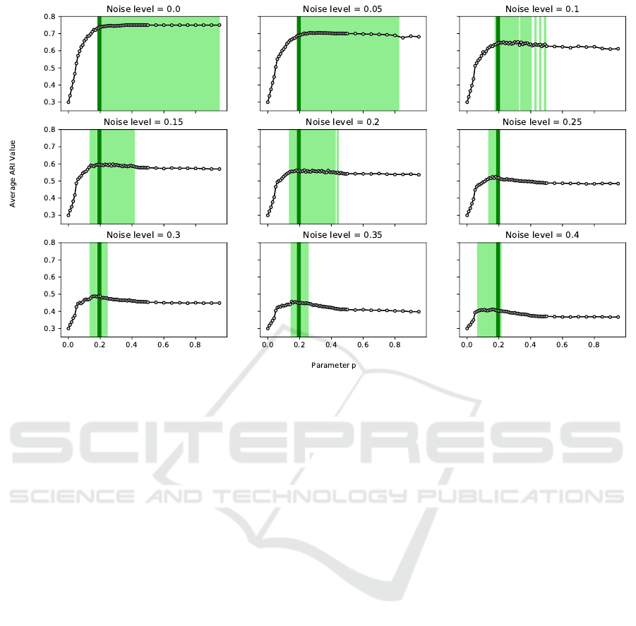
Figure 1: The nine plots visualize the relationship between parameter p and the ARI value averaged across data sets and

repetitions for the nine constraint sets with different noise levels. The range of penalty values that led to average ARI values

that are within 2.5% of the highest average ARI value obtained for the respective noise level are highlighted in light green.

The intersection of the light green ranges is highlighted in dark green.

are some data sets where values for parameter p that

are close to zero deliver the best ARI values for noisy

constraint sets. These are often data sets where the

original (unconstrained) k-means algorithm already

performs well. For those data sets, adding ML and

CL constraints is often only helpful if the constraints

are noise-free. With p = 0, the BH-kmeans algorithm

corresponds to the standard (unconstrained) k-means

algorithm.

Next, we analyze the relationship between pa-

rameter p and the average running time in seconds.

The nine plots in Figure 2 visualize the relationship

between parameter p and the average running time

across all data sets and repetitions for the nine con-

straint sets with different noise levels. The running

time tends to increase with increasing value of pa-

rameter p and increasing noise level. However, the

overall impact of parameter p on the running time is

moderate. A value of p ∈ [0.18, 0.20] is also a good

choice with respect to running time.

6 CONCLUSIONS

Despite the great algorithmic advances in integer op-

timization during the last 25 years, the use of mixed-

integer optimization is still relatively rare in con-

strained clustering. This paper demonstrates the po-

tential of mixed-integer optimization in this ﬁeld. We

propose a variant of the k-means algorithm that uses

mixed-integer optimization to incorporate ML and CL

constraints as soft constraints that can be violated sub-

ject to a penalty. The performance of our algorithm on

a large set of benchmark instances is superior to that

of the state-of-the-art algorithm. We also provided

guidelines on how to determine the penalty value for

violating constraints when the ML and CL constraints

are noisy.

Inspired by the results reported here, we extended

the BH-kmeans algorithm such that the user can spec-

ify individual penalties for ML and CL constraints.

This feature is useful in situations where the experts

state ML and CL constraints with different levels of

conﬁdence. In the extended version, the user can

additionally deﬁne a subset of pairwise constraints

that will be treated as hard constraints. The extended

version also includes a preprocessing procedure that

contracts objects that are transitively connected by

hard ML constraints and a technique that reduces the

number of variables and constraints in the mixed-

binary linear programming formulation. Due to lack

of space, we will present the features of the extended

version together with computational results in another

paper.

A k-Means Algorithm for Clustering with Soft Must-link and Cannot-link Constraints

201

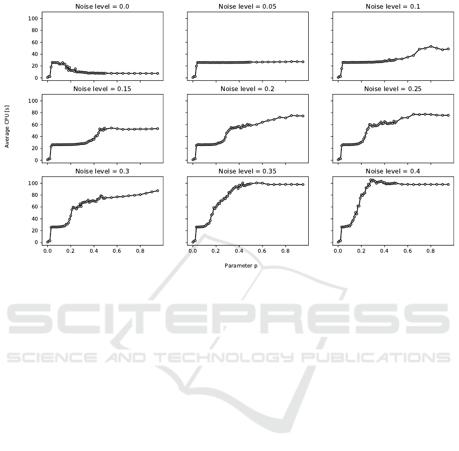
Figure 2: The nine plots visualize the relationship between parameter p and the running time averaged across data sets and

repetitions for the nine constraint sets with different noise levels.

REFERENCES

Antoine, V., Quost, B., Masson, M.-H., and Denoeux, T.

(2012). Cecm: Constrained evidential c-means al-

gorithm. Computational Statistics & Data Analysis,

56(4):894–914.

Arthur, D. and Vassilvitskii, S. (2007). k-means++: The ad-

vantages of careful seeding. In Gabow, H., editor, Pro-

ceedings of the Eighteenth Annual ACM-SIAM Sym-

posium on Discrete Algorithms, pages 1027–1035,

Philadelphia, Pennsylvania USA.

Basu, S., Banerjee, A., and Mooney, R. J. (2004). Active

semi-supervision for pairwise constrained clustering.

In Proceedings of the 2004 SIAM international con-

ference on data mining, pages 333–344. SIAM.

Baumann, P. (2020). A binary linear programming-based

k-means algorithm for clustering with must-link and

cannot-link constraints. In 2020 IEEE International

Conference on Industrial Engineering and Engineer-

ing Management (IEEM), pages 324–328. IEEE.

Davidson, I. and Ravi, S. (2005). Clustering with con-

straints: Feasibility issues and the k-means algorithm.

In Proceedings of the 2005 SIAM international con-

ference on data mining, pages 138–149. SIAM.

de Oliveira, R. M., Chaves, A. A., and Lorena, L. A. N.

(2017). A comparison of two hybrid methods for con-

strained clustering problems. Applied Soft Computing,

54:256–266.

Ganji, M., Bailey, J., and Stuckey, P. J. (2016). La-

grangian constrained clustering. In Proceedings of the

2016 SIAM International Conference on Data Mining,

pages 288–296. SIAM.

Gonz

alez-Almagro, G., Luengo, J., Cano, J.-R., and Garc

ıa,

S. (2020). DILS: constrained clustering through dual

iterative local search. Computers & Operations Re-

search, 121:104979.

Khashabi, D., Wieting, J., Liu, J. Y., and Liang, F. (2015).

Clustering with side information: From a probabilis-

tic model to a deterministic algorithm. arXiv preprint

arXiv:1508.06235.

Lampert, T., Dao, T.-B.-H., Lafabregue, B., Serrette,

N., Forestier, G., Cr

emilleux, B., Vrain, C., and

Ganc¸arski, P. (2018). Constrained distance based clus-

tering for time-series: a comparative and experimen-

tal study. Data Mining and Knowledge Discovery,

32(6):1663–1707.

Pelleg, D. and Baras, D. (2007). K-means with large and

noisy constraint sets. In European Conference on Ma-

chine Learning, pages 674–682. Springer.

Wagstaff, K., Cardie, C., Rogers, S., Schr

odl, S., et al.

(2001). Constrained k-means clustering with back-

ground knowledge. In Proceedings of the Eigh-

teenth International Conference on Machine Learn-

ing, pages 577–584.

Wu, B., Zhang, Y., Hu, B.-G., and Ji, Q. (2013). Con-

strained clustering and its application to face cluster-

ing in videos. In Proceedings of the IEEE conference

on Computer Vision and Pattern Recognition, pages

3507–3514.

ICPRAM 2022 - 11th International Conference on Pattern Recognition Applications and Methods

202