
Clustering Quality of a High-dimensional Service Monitoring
Time-series Dataset
Farzana Anowar
1,2 a
, Samira Sadaoui
1 b
and Hardik Dalal
2
1
University of Regina, Regina, Canada
2
Ericsson Canada Inc., Montreal, Canada
Keywords:
High-dimensional Time-series Dataset, Clustering Quality, Data Clustering, Data Imputation, Deep Learning.
Abstract:
Our study evaluates the quality of a high-dimensional time-series dataset gathered from service observability
and monitoring application. We construct the target dataset by extracting heterogeneous sub-datasets from
many servers, tackling data incompleteness in each sub-dataset using several imputation techniques, and fusing
all the optimally imputed sub-datasets. Based on robust data clustering approaches and metrics, we thoroughly
assess the quality of the initial dataset and the reconstructed datasets produced with Deep and Convolutional
AutoEncoders. The experiments reveal that the Deep AutoEncoder dataset’s performances outperform the
initial dataset’s performances.
1 INTRODUCTION
In industry, an incredible amount of data is produced
on a daily basis (Anowar and Sadaoui, 2021a; Anowar
and Sadaoui, 2020). Sometimes, data are not appro-
priately captured, which may be caused by human er-
rors, or sensor malfunction, resulting in data incom-
pleteness (i.e., missing values). Additionally, in the
presence of high dimensionality in the data, the train-
ing process becomes complicated for Machine Learn-
ing Algorithms (MLAs), leading to the model over-
fitting and lowering the predictive performance (Jin-
dal and Kumar, 2017), (Anowar and Sadaoui, 2021b).
These two issues become more critical for time-series
datasets since the latter are collected over large time
frames. As a consequence, there are much more
chances of having missing values and high dimen-
sionality, which necessitate special attention from the
experts when dealing with these data (Rani and Sikka,
2012).
Based on an industrial application, we construct
a new End-to-End (E2E) service monitoring time-
series dataset so that users (developers, DevOps engi-
neers, IT managers, and site reliability engineers) can
respond to system-wide performance changes, mon-
itor the services’ availability, and optimize the re-
source utilization. For this purpose, we first collect
a
https://orcid.org/0000-0002-1535-7323
b
https://orcid.org/0000-0002-9887-1570
data from multiple sub-servers over six weeks. How-
ever, the collected sub-datasets are heterogeneous in
terms of feature spaces and sizes. Before merging
the sub-datasets, we address the issue of data in-
completeness for each sub-dataset separately. We
tackle missing values with several imputation tech-
niques carefully and keep the optimally imputed sub-
datasets only. Subsequently, we fuse the imputed
sub-datasets based on the time-stamp feature to pro-
duce the final time-series service monitoring dataset.
The latter is unlabelled, temporal, and high dimen-
sional. Since the dataset is new and complex, we
need to evaluate its quality before using it for any
decision-making task. This study compares several
clustering techniques on this very high-dimensional
dataset and its reconstructed equivalent datasets. To
this end, first, we handle the high dimensionality is-
sue and second adopt data clustering methods, in-
cluding two conventional and two recent time series-
based algorithms, in which the dataset is divided into
several optimal groups. Since high dimensional data
brings computational challenges for developers, we
use Deep and Convolutional Autoencoders to improve
our dataset’s quality and then assess the quality of
the reconstructed datasets using the same clustering
methods.
Many efficient dimensionality reduction methods
reduce the feature space effectively; however, they are
unable to recover the original data (Anowar et al.,
2021). In contrast, the AutoEncoders are effective
Anowar, F., Sadaoui, S. and Dalal, H.
Clustering Quality of a High-dimensional Service Monitoring Time-series Dataset.
DOI: 10.5220/0010801400003116
In Proceedings of the 14th International Conference on Agents and Artificial Intelligence (ICAART 2022) - Volume 2, pages 183-192
ISBN: 978-989-758-547-0; ISSN: 2184-433X
Copyright
c
2022 by SCITEPRESS – Science and Technology Publications, Lda. All rights reserved
183

not only in lowering the dimensionality but also in
reconstructing the original data. We also make sure
not to lose much information while reconstructing
the data. Lastly, we thoroughly compare the qual-
ity of the initial and reconstructed datasets based on
the optimal clusters using several quality metrics to
show the efficacy of the reconstructed datasets. The
obtained best clusters will be used for any further
decision-making tasks in the ML domain. We uti-
lize AutoEncoders to showcase that the reconstructed
feature space yields better clustering than the orig-
inal dataset. Our experimental results demonstrate
that the clustering performances of the reconstructed
dataset with Deep AutoEncoder (DAE) increased sig-
nificantly over the clustering performances with the
initial dataset. To the best of our knowledge, no prior
research provided a thorough analysis of the cluster-
ing quality of a high-dimensional time-series dataset
that comes with missing values.
We structure the paper as follows. Section 2 dis-
cusses recent data clustering methods for assessing
the quality of high dimensional datasets. Section 3
presents the preprocessing and the fusion process to
build the target datasets. Section 4 describes the clus-
tering approaches and their quality evaluation metrics.
Section 5 develops two deep learning methods to re-
construct the dataset. Section 6 and Section 7 perform
several experiments to assess the clustering quality of
the initial and reconstructed datasets. Section 8 com-
pares all the clustering quality results. Section 9 con-
cludes our work with future work.
2 RELATED WORK
We examine notable studies that utilized diverse data
clustering methods to deal with high-dimensional
datasets specifically and reduce their complexity. For
instance, the authors in (Dash et al., 2010) combined
the dimensionality reduction method named Princi-
pal Component Analysis (PCA) and the data clus-
tering technique K-means. First, to make K-means
more effective, they proposed to utilize the instances
that have the maximum squared Euclidian distance
(among all the instances) as the initial centroids for
the clustering task. Next, they compared the perfor-
mances of the original K-means and the new pro-
posed approach using the reduced PCA dataset. They
showed that the results produced with the proposed
centroid selection method are more accurate, easy to
visualize, and the time complexity was substantially
decreased.
Any feature selection technique for high dimen-
sional datasets is assessed from two perspectives
(Song et al., 2011): efficiency and effectiveness,
where efficiency is related to the time required to
obtain the optimal sub-group of features, and ef-
fectiveness concerns the quality of this sub-group.
A fast clustering-based feature selection approach is
proposed in (Song et al., 2011), which operates in
two phases. Firstly, all the features are partitioned
into clusters based on the ”graph-theoretic cluster-
ing” technique to select the subsets of features, and
secondly, from each cluster, the most relevant fea-
ture that is closely connected to the target variable
is chosen again to provide the best selection of fea-
tures. The authors adopted the clustering method
called ”Minimum-Spanning Tree” to prove the com-
petence of the proposed method and carried out ex-
periments to evaluate the performances between the
proposed method and several existing feature selec-
tion algorithms. The experiments demonstrated that
the proposed approach returned reduced subsets of
features and improved the performances of the clas-
sification task.
For tackling the data dimensionality, Feature Se-
lection Algorithms (FSAs) were mainly adopted in
the literature. However, FSAs fail for large-scale fea-
ture spaces. Hence, the authors in (Chormunge and
Jena, 2018) addressed this problem by integrating a
clustering technique with a correlation measure to
generate a good subset of features. They first elim-
inated the insignificant features using K-means clus-
tering, and later, the non-redundant features are cho-
sen by utilizing the correlation metric from each clus-
ter. For the experimental purpose, they used microar-
ray and text datasets to evaluate the proposed method
and compared the performances with two other FSAs,
ReliefF and Information Gain, using the Na
¨
ıve Bayes
classifier. The experimental results showed that the
most representative features were chosen by varying
the number of relevant features and provided better
accuracy than the other two FSAs.
Detecting outliers is an essential ML task because
outliers may carry important information. However,
in the case of high-dimensional datasets, outliers may
lead to worse performances. Therefore, the authors
in (Messaoud et al., 2019) developed a hybrid frame-
work named ‘Infinite Feature Selection DBSCAN’
(InFS-DBSCAN) to decrease the dimensionality of
datasets and identify outliers efficiently using cluster-
ing techniques. They first removed insignificant fea-
tures by selecting the k-most relevant features from
the high dimensional data space and then adopted
the DBSCAN algorithm to detect outliers. Two real-
world datasets were used for the experiments to com-
pare the performances of the proposed approach with
DBSCAN and FS-DBSCAN clustering in terms of the
ICAART 2022 - 14th International Conference on Agents and Artificial Intelligence
184

clustering accuracy and error rate. For both datasets,
the proposed approach outperformed the other meth-
ods.
3 TIME-SERIES DATASET
CONSTRUCTION
The data we use for the experiments was collected
through Prometheus from October 26 to December
03, 2020, every 15 seconds for many available ser-
vices. The data is extracted from a monitoring service
that comes with three critical characteristics:
1. By nature data is high dimensional and temporal
(time series).
2. Data was collected from different sub-servers, so
it is stored and processed separately.
3. Data has many missing values due to the nature
of the applications hosted on the servers and net-
work/hardware/software failures.
More precisely, we retrieve data from 48 sub-
servers (in CSV format). The extracted sub-datasets
possess different sizes and sets of features. Af-
ter examining all the data, we found two types:
Counter and Gauge. The Counter type indicates a
single monotonically growing counter whose value
can either increase or be reset to zero on restart
(Prometheus, 2021). The Gauge type denotes a single
numerical value that can arbitrarily go up and down
(Prometheus, 2021).
3.1 Handling Missing Values in Each
Sub-server Data
Nevertheless, all the sub-server files contain missing
values. There are several options to tackle those val-
ues, such as imputation, removal of data with miss-
ing values (good option only when missing values are
rare), replacement with constant values (i.e. 0 or 1).
The last two options are not practical if many miss-
ing values are present, like in some of our sub-servers
files. Hence, we choose three imputation techniques:
(1) KNN Imputation, (2) MissForest Imputation, and
(3) SimpleImputer using the mean value. KNN im-
putation is easy to implement and fast, MissForest
can handle mixed data type (numerical and categori-
cal) and works efficiently with high-dimensional data,
and SimpleImputer performs much faster and can also
tackle mixed data. (Jadhav et al., 2019), (Pedregosa
et al., 2011), (Stekhoven and B
¨
uhlmann, 2012).
We apply the three techniques to each sub-server
dataset separately to obtain relevant imputed values.
Table 1: Silhouette-Index Scores for Data Imputation.
Sub-server SimpleImputer KNN MissForest
#1 0.996663641 0.996662706 0.995631504
#3 0.932876262 0.932890974 0.932648194
#4 0.493330594 0.523756138 0.549322423
Furthermore, we utilize the “Silhouette Index” to as-
sess the new values. The imputation method that re-
turns the best (higher) Silhouette score is selected for
each file. Table 1 reports the Silhouette scores for
three sub-servers, as examples. For different sub-
server files, different methods are needed to achieve
the best data quality. Indeed, we obtain 31 opti-
mally imputed sub-datasets with SimpleImputer, 4
optimally imputed data with KNN imputation, and
13 optimally imputed data with MissForest. We
may note that MisssForest necessitated more compu-
tational time than the two others.
3.2 Fusing Heterogeneous Sub-server
Datasets
As mentioned earlier, we obtain 48 optimally imputed
sub-datasets. Subsequently, we conduct the “Inner
Join” procedure to merge the many heterogeneous
sub-datasets by considering the time-stamp column
as the key component. This procedure keeps the in-
stances from the participating files as long as there
is a match between the key columns. It returns all
the rows where the key component (here time-stamp)
of one file is equal to the key records of another file.
As a result, we produce the final E2E service moni-
toring dataset consisting of 3,100 features and 53,953
instances over 6 weeks (39 days). This dataset is of a
large scale and highly dimensional.
We use a simple example to explain the Inner
Join procedure (Figure 1) where we have two sepa-
rate databases: Product and Customer. After apply-
ing Inner Join to both files using the ProductID as
the key column, we obtain only 1 row (with 10 fea-
tures) as the two files have only one common value
(101). Also, notice that the attribute City is present
in both databases, and Inner Join produces 2 different
attributes (City x and City y) for the final output, as
the first one denotes the product’s warehouse location
and the second one is the delivery location.
Figures 2 and 3 plot two features named ‘Re-
quests1’ and ‘Responses1’ (selected randomly) from
the E2E service monitoring dataset. In Figure 2, data
has either went up or is set to 0, which implies that
the feature ‘Request1’ contains Counter-type data. In
Figure 3, data has gone up and down arbitrarily, which
shows that the feature ‘Responses1’ is of the Gauge
type.
Clustering Quality of a High-dimensional Service Monitoring Time-series Dataset
185
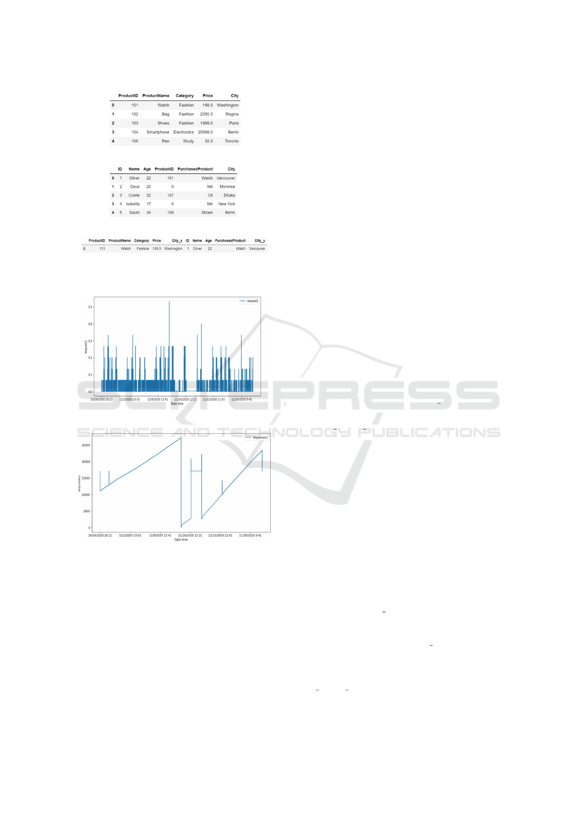
(a) Product DB.
(b) Customer DB.
(c) Inner Join of Product and Customer.
Figure 1: Concept of Inner Join.
Figure 2: Feature ‘Request1’ (Counter Type).
Figure 3: Feature ‘Responses1’ (Gauge Type).
3.3 Normalizing the New Feature Space
After examining the final dataset, we observe that
most features (80.64%) have quite small values, and
19.36% of features have very high values. The big
value disparities between features require to re-scale
the entire dataset. Using the min-max scaler in
Python, we try multiple ranges, including [0-1], [0-
10], [0-50], [0-100] for the AutuEncoders’ loss opti-
mization, and obtain [0-1] is the best range to re-scale
the dataset for the experiment.
4 CLUSTERING APPROACHES
AND METRICS
We assess the quality of the new dataset through un-
supervised learning using data clustering since it is
unlabeled. It is critical for any unsupervised ML task
to obtain high-quality clusters in order to find the hid-
den patterns or unknown correlations in a dataset (Wu
et al., 2020). To this end, we select different clus-
tering techniques: partition-based, time-series-based,
and density-based, described below:
• K-means is a widely employed clustering
technique in the literature (Niennattrakul and
Ratanamahatana, 2007), (Aghabozorgi et al.,
2015).
• TS-Kmean and TS-Kshape are both designed ex-
plicitly for time series with a high dimensionality
(Tavenard et al., 2020). The specialty about TS-
Kmean is that it can weigh the time-stamps au-
tomatically based on the time-span’s significance
during the clustering operation (Huang et al.,
2016). TS-Kshape computes the distance mea-
sure and centroids using the normalized cross-
correlation of two time series for each iteration,
and update the assignments of the clusters (Pa-
parrizos and Gravano, 2015). Both methods have
only one hyper-parameter (max iter).
• HDBSCAN has one hyper-parameter
(min cluster size) compared to other density-
based methods. It can handle highly dense data,
like ours. Besides, it can tackle the varying den-
sity issue, which the standard DBSCAN method
cannot (Saul, 2017). Additionally, HDBSCAN
does not require knowing the count of clusters
beforehand, unlike the three previous methods
(McInnes and Healy, 2017).
A well-known fact about K-means is that it
takes more time to converge for large-scale datasets
(Prabhu and Anbazhagan, 2011), like ours. To fix
this issue, we utilize K-means++ as the initializer in-
side the K-means algorithm to make the convergence
much faster. For utilizing TS-Kmean and TS-Kshape,
we first import ‘tslearn’, a Python machine learn-
ing package for time-series datasets. Also, for TS-
Kmean, we set max iter to 50 and include the ini-
tializer K-means++ as well, and for the cluster as-
signments, we use the Euclidean distance. More-
over, for TS-Kshape, we set max iter to 100. For the
three first methods, we search for the optimal number
of clusters using Elbow, Silhouette Coefficient, and
Caliniski-Harabasz (CH) Index. Lastly, we allocate
min cluster size to 2000 for HDBSCAN, as we be-
lieve out of 53,953 data, the minimum 2000 data (≈
ICAART 2022 - 14th International Conference on Agents and Artificial Intelligence
186

26%) for a cluster is good enough.
To assess the quality of the produced clusters by
the four methods, we utilize the following quality
metrics, described below:
• Sum of Squared Error (SSE) that identifies how
internally coherent each cluster is. The lower the
SSE, the better the cluster is (Pedregosa et al.,
2011).
• Davies-Bouldin (DB) Index that defines the aver-
age similarity of each cluster, i.e., the intra-cluster
distance should be minimum. Hence the lower,
the better (Pedregosa et al., 2011).
• Variance Ratio Criterion (VRC) that quantifies the
ratio of “between-cluster dispersion” and “within-
cluster dispersion”. The higher the VRC, the bet-
ter the cluster is (Zhang and Li, 2013).
We compute the performances of all the opti-
mal clusters for the initial dataset and reconstructed
datasets. To this end, we utilize SSE, DB, and VRC
for K-means, TS-Kmean and TS-Kshape, and only
DB and VRC for HDBSCAN, as the latter doesn’t
have the SSE object in Python.
5 RECONSTRUCTED DATASETS
WITH AUTOENCODERS
Since numerous services run on the servers’ side,
data are generated at high speed and with soaring
dimensionality. Consequently, we adopt two self-
supervised deep-learning methods to improve the data
quality: Deep AutoEncoder (DAE) and Convolutional
AutoEncoder (ConAE). AutoEncoders uses encoder
and decoder layers. The former uses a latent space
to compress the inputs, and the later reconstructs the
original dataset as closely as possible from this com-
pressed data(Wang et al., 2016). Autoencoders learn
from the data while back-propagating the neural net-
work by disregarding insignificant data during encod-
ing, resulting in a better-reconstructed dataset (Law-
ton, 2020). Furthermore, the goal of training Au-
toEncoders is to minimize the reconstruction loss; the
lower the reconstruction loss, the more similar the
reconstruction of the original data can be generated
(Wang et al., 2016). Thanks to these methods, we do
not worry about reducing the high feature space opti-
mally.
The main challenge is determining the optimal ar-
chitecture for our complex service monitoring dataset.
We first develop the DAE using a deep, fully con-
nected neural network. We try several rigorous com-
binations of hidden layers, loss function, weight op-
timizer, activation functions, epochs and batch sizes.
(a)
(b)
Figure 4: Loss for Different Combinations of DAE.
For instance, if we utilize 10 hidden layers for both
encoder and decoder, MSE as the loss function, Adam
as the optimizer, Relu as the activation function, batch
size of 256 with 3500 epochs, the obtained loss is high
(more than 0.45) as shown in Figure 4 (a). On the
other hand, if we use only one hidden layer for both
encoder and decoder, SGD as the optimizer, Sigmoid
as the activation function, batch size of 512 with 50
epochs, we obtain a negative loss as depicted in Fig-
ure 4 (b).
The best architecture that we attain for DAE com-
prises 6 hidden layers for both encoder and decoder,
1032 for batch size, Adadelta as the optimizer, Relu
for all the hidden layers, Sigmoid for the output layer
as activation function, and MSE as the loss function.
More precisely, for the encoder part, we sequentially
provide 3100 (original), 2500, 1650, 1032, 500, 100
and 5 features using six hidden layers, and again, we
reconstruct the features from 5, 100, 500, 1032, 1650,
2500 and 3100.
Regarding ConAE, we build a sequential neu-
ral network with two hidden layers for both encoder
and decoder. For the encoder layers, we utilize the
Conv1D class with 128 and 16 filters, and for the de-
coder layers, Conv1D with 16 and 128 filters; the ker-
nel size of all the filters is 3. For the encoding layers,
we use MaxPooling1D with a pool size of 2 to down-
sample the input representation. We adopt UpSam-
pling1D with size of 2 for the decoder to upsample
the input representation from the encoder. Also, keep
in mind that the output of ConAE is a 3D array; hence,
it needs to be converted to a 2D array before using it
for subsequent experiments.
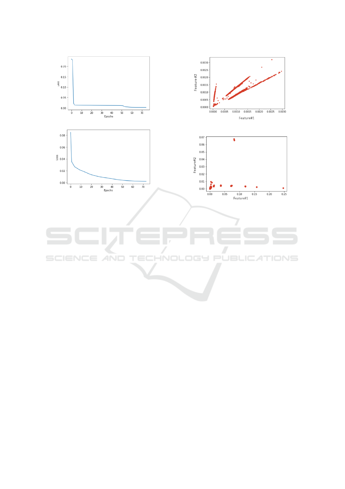
Besides, we use five consecutive epochs with no
reduction by 0.0001 as the stopping criterion for train-
ing, and the reconstruction error for DAE is 0.0016
with the 75th epoch out of 100 epochs. However,
Clustering Quality of a High-dimensional Service Monitoring Time-series Dataset
187
(a)
(b)
Figure 5: Loss Graph for DAE (a) and ConAE (b).
while implementing ConAE, the critical challenge is
the computational complexity. Thus, instead of 5
consecutive epochs, we choose 3 without reducing
loss by 0.0001 as the stopping criterion. We obtain
the reconstruction error of 0.0021 and optimal epoch
of 74. Here, for both DAE and ConAE, the iter-
ations stop at 75th and 74th epochs respectively as
they meet the stopping criterion. We present the loss
graphs for DAE and ConAE in Figure 5 where the loss
curve goes steep down drastically after three epochs
for DAE in Figure 5(a) and gradually goes down for
ConAE in Figure 5(b). Furthermore, Figures 6 and
7 illustrate the reconstructed datasets with the first
two features that we obtain after utilizing DAE and
ConAE models. In Figure 6, data are scattered across
the distribution, and in contrast, in Figure 7, data are
more densely located in similar positions.
Nevertheless, one crucial question raises while
compressing the initial dataset with DAE and ConAE
is that how much information was lost. For this pur-
pose, we employ the reconstruction error to measure
the information loss. As mentioned earlier, we obtain
the reconstruction error of 0.0016 and 0.0021, respec-
tively, for the reconstructed datasets using DAE and
ConAE, which are very minimal. Hence, we can con-
clude that with deep-learning methods, we lost a very
minimum amount of information.
Figure 6: Reconstructed Dataset using DAE.
Figure 7: Reconstructed Dataset using ConAE.
6 CLUSTERING QUALITY OF
INITIAL DATASET
First, we utilize Elbow method, Silhouette coefficient
and CH Index to search for the best number of clus-
ters for the initial dataset, as presented in Table 2, and
Elbow, Silhouette and CH Index are described below:
1. Elbow method: One of the most popular tech-
niques for identifying the optimal number of clus-
ters. It is based on the calculation of “Within-
Cluster-Sum of Squared (WSS)” errors for a dif-
ferent number of clusters (k). It iterates over the k
and calculates the WSS errors (Yuan and Yang,
2019). Small values indicate that clusters are
more likely to be convergent, and after reaching
the optimal cluster’s number, WSS error starts de-
clining (Yuan and Yang, 2019).
2. Silhouette coefficient: This metric calculates
the cluster’s cohesion and separation (Pedregosa
et al., 2011). It measures how well an instance
fits into its corresponding cluster. The values of
the Silhouette coefficient range between -1 and 1
(Pedregosa et al., 2011). A high (close to 1) sil-
houette score indicates that data are closer to their
assigned clusters than others. A score close to 0
means that data is very close to or on the deci-
sion boundary between two neighboring clusters.
A score close to -1 means that data is probably as-
ICAART 2022 - 14th International Conference on Agents and Artificial Intelligence
188

Table 2: Optimal Cluster Numbers.
Dataset
Optimal Clustering
Initial Dataset
Elbow Silhouette CH
5 5 4
Reconstructed Dataset
with DAE
Elbow Silhouette CH
5 6 14
Reconstructed Dataset
with ConAE
Elbow Silhouette CH
5 5 5
signed to a wrong cluster (Kaoungku et al., 2018).
3. CH Index: The basic idea of CH index is that
clusters that are very compact and well-separated
from each other are good clusters. This index is
a metric that compares how similar a cluster’s in-
stance is to that than other clusters (Wang and Xu,
2019).
Then, we fed the optimal number of clusters from
Table 2 to the three clustering methods (K-means, TS-
Kmeans and TS-Kshape). We do not supply the num-
ber of clusters to HDBSCAN, as by default it pro-
duces this number (which is 6). We report the per-
formances of the four clustering methods in Table 3,
with a tally of 20 results. We attain the minimum SSE
(0.004348) with TS-Kshape using 5 clusters, the min-
imum DB (0.61332) with K-means using 4 clusters.
K-means with 4 clusters provides the maximum VRC
(103431.341). However, the data performance with
HDBSCAN is not satisfactory. Due to the high data
density, we present the 3-D visualization of two ex-
amples of optimal clusters in Figure 8 to have a much
better graphical representation where x, y ans z axes
represent the first three dimensions: dimension#1, di-
mension#2, and dimension#3.
Table 3: Optimal Clustering Quality of Initial Dataset.
K-means
5 clusters 4 clusters
SSE DB VRC SSE DB VRC
245568.441 0.613830 102604.2395 313075.295 0.61332 103431.341
TS-Kmean
5 clusters 4 clusters
SSE DB VRC SSE DB VRC
4.9938 0.613830 102604.2395 5.80274 0.7040410 97865.0800
TS-Kshape
5 clusters 4 clusters
SSE DB VRC SSE DB VRC
0.004348 2.243981 75912.984 0.00716 0.70334 62285.962
HDBSCAN with 6 clusters
DB VRC
1.3517 80707.7806
7 CLUSTERING QUALITY OF
RECONSTRUCTED DATASETS
Table 2 exposes the optimal clustering for the recon-
structed datasets. For the ConAE dataset, all the tech-
niques (Elbow, Silhouette and CH) return the same
number, unlike for the DAE dataset. Elbow tech-
nique yields the same optimal clustering for the three
datasets. However, CH recommends different cluster-
ing numbers, especially for the DEA datasets. Most
of the numbers are close by, except one (14), and
among the nine results, six return the number 5. Since
the reconstructed DAE dataset is sparsely separated
over the feature-space, CH Index returns a higher ra-
tio of between and within cluster sums of squares, re-
sulting in a higher (14) optimal clustering.
Next, Table 4 evaluates the optimal cluster qual-
ity for the DEA reconstructed dataset, with a tally of
20 results. We obtain the lowest SSE of 0.0019202
with TS-Kshape using 14 clusters, the minimum DB
of 0.05016857 with K-means and TS-Kmeans using
6 clusters, and the highest VRC of 30,312,918.2572
with K-means using 14 clusters. A higher VRC score
implies that the clusters are dense (minimized intra-
cluster distance) and well separated (maximized inter-
cluster distance) (Pedregosa et al., 2011). Table 5 as-
sesses the quality of the ConAE reconstructed dataset.
The lowest SSE of 0.004682736 is achieved with
TS-Kshape, the minimum DB with of 0.61332691
with both K-means and TS-Kmean, and the highest
VRC of 95738.59064 with K-means. Across the three
datasets, HDBSCan under-performs.
(a) K-means with Four Clusters.
(b) TS-Kshape with Five Clusters.
Figure 8: Two Examples of Optimal Clusters of Initial
Dataset.
Clustering Quality of a High-dimensional Service Monitoring Time-series Dataset
189
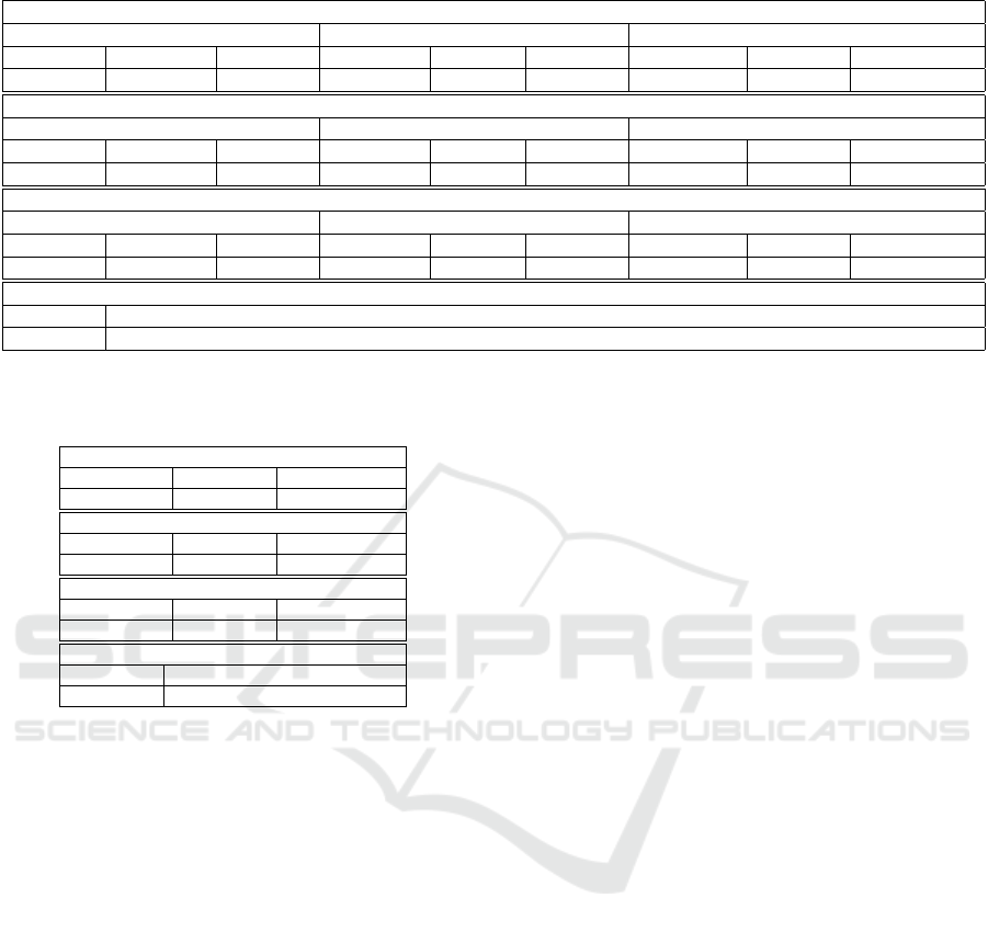
Table 4: Quality of DAE Reconstructed Dataset.
Kmeans
Elbow-5 clusters Silhouette-6 clusters CH-14 clusters
SSE DB VRC SSE DB VRC SSE DB VRC
16807.5332 0.181151753 1510548.891 1252.5371 0.05016857 16349947.76 259.94039 0.5234089 30312918.2572
TS-Kmean
Elbow-5 clusters Silhouette-6 clusters CH-14 clusters
SSE DB VRC SSE DB VRC SSE DB VRC
0.31155592 0.18115175 1510548.89 0.023216931 0.05016857 16349947.76 0.00497385071 0.482265234 28591306.875589
TSKshape
Elbow-5 clusters Silhouette-6 clusters CH-14 clusters
SSE DB VRC SSE DB VRC SSE DB VRC
0.002113596 0.4164552564 50036.65944 0.0019847939 0.43711877 315043.8333 0.0019202 0.4703590 16066475.8277
HDBSCAN-6 clusters
DB VRC
1.026604381 12825430.68
Table 5: Quality of ConAE Reconstructed Dataset (5 Clus-
ters).
K-means
SSE DB VRC
270260.4375 0.61332691 95738.59064
TS-Kmean
SSE DB VRC
6.316888253 0.61332691 73127.0153677
TS-Kshape
SSE DB VRC
0.004682736 1.7982134 71203.693461
HDBSCAN-5 clusters
DB VRC
1.18025933 76806.51995
8 COMPARISON
Table 6 compares the clustering performances be-
tween the initial dataset and the two reconstructed
datasets. All the metric results of the DAE recon-
structed dataset outperform the outcome attained with
the initial dataset due to the non-linear properties
of the activation functions. The gap between the
SSE values equals 0.0024 (minimal), between the
DB values 0.56316 (high), and between VRC values
30,209,486.919 (very high).
In contrast, for the ConAE reconstructed dataset,
we observe that all performance metrics are under-
performing due to the convolutional layer that could
not handle the non-linear time-series dataset. Nev-
ertheless, the ConAE metrics are pretty close to the
metrics obtained with the initial dataset.
In conclusion, the DEA dataset possesses the
highest quality. Moreover, for the SSE metric, the
TS-Kshape is the dominant clustering method across
the three datasets. For the DB and VRC metrics, K-
means is the most performing method. Also, 14 rep-
resents the best cluster number. For conducting the
subsequent decision-making tasks, the DEA dataset
based on K-means with 14 clusters will be provided to
the industrial partner, as the latter provides a large gap
between the VRC values. Furthermore, we visualize
all the best clustering performances for the DEA re-
constructed dataset in Figure 9 where each cluster ori-
entation is different from others for TS-Kshape, TS-
Kmeans and K-means.
9 CONCLUSIONS AND FUTURE
WORK
Our study first constructed a high-dimensional time-
series dataset. However, this new dataset should
be of high quality as it will be utilized for essen-
tial decision-making tasks by the industrial partner.
We jointly addressed two significant problems of this
dataset: data incompleteness and high dimensional-
ity. We thoroughly assessed the quality of the initial
dataset and reconstructed datasets produced with self-
supervised deep learning networks using several data
clustering approaches. The experiments showed a
higher quality for the reconstructed dataset with DAE
when using a higher number of clusters.
A crucial research direction of our study is to ex-
plore clustering-based outlier detection of the recon-
structed datasets.
ACKNOWLEDGEMENTS
We cordially thank the Observability team for grant-
ing us access to the data.
ICAART 2022 - 14th International Conference on Agents and Artificial Intelligence
190
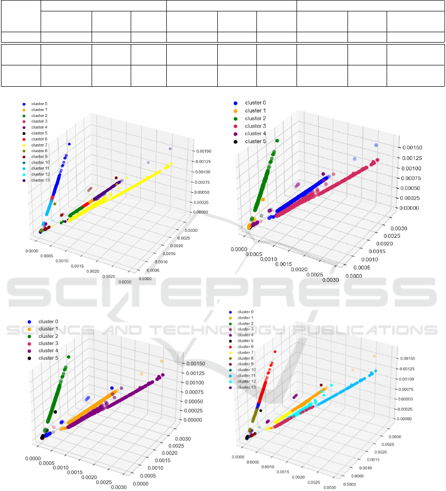
Table 6: Comparison based on Clustering Performances.
Dataset
Metric 1 Metric 2 Metric 3
Clustering
Algo.
Cluster
No.
SSE
Clustering
Algo.
Cluster
No.
DB
Clustering
Algo.
Cluster
No.
VRC
Initial TS-Kshape 5 0.0043 K-means 4 0.61332 K-means 4 103431.341
DAE TS-Kshape 14 0.0019
K-means
TS-Kmean
6 0.05016 K-means 14 30312918.26
ConAE TS-Kshape 5 0.0046
K-means
TS-Kmean
5 0.61336 K-means 5 95738.59
(a) TS-Kshape with 14 clusters. (b) TS-Kmean with 6 clusters.
(c) K-means with 6 clusters. (d) K-means with 14 clusters.
Figure 9: Optimal Clusters for DEA Reconstructed Dataset.
REFERENCES
Aghabozorgi, S., Shirkhorshidi, A. S., and Wah, T. Y.
(2015). Time-series clustering–a decade review. In-
formation Systems, 53:16–38.
Anowar, F. and Sadaoui, S. (2020). Incremental neural-
network learning for big fraud data. In 2020 IEEE
International Conference on Systems, Man, and Cy-
bernetics (SMC), pages 3551–3557.
Anowar, F. and Sadaoui, S. (2021a). Incremental learn-
ing framework for real-world fraud detection environ-
Clustering Quality of a High-dimensional Service Monitoring Time-series Dataset
191

ment. Computational Intelligence, 37(1):635–656.
Anowar, F. and Sadaoui, S. (2021b). Incremental learning
with self-labeling of incoming high-dimensional data.
In The 34th Canadian Conference on Artificial Intel-
ligence, pages 1–12.
Anowar, F., Sadaoui, S., and Selim, B. (2021). Conceptual
and empirical comparison of dimensionality reduction
algorithms (pca, kpca, lda, mds, svd, lle, isomap, le,
ica, t-sne). Computer Science Review, 40:1–13.
Chormunge, S. and Jena, S. (2018). Correlation based
feature selection with clustering for high dimensional
data. Journal of Electrical Systems and Information
Technology, 5(3):542–549.
Dash, B., Mishra, D., Rath, A., and Acharya, M. (2010). A
hybridized k-means clustering approach for high di-
mensional dataset. International Journal of Engineer-
ing, Science and Technology, 2(2):59–66.
Huang, X., Ye, Y., Xiong, L., Lau, R. Y., Jiang, N., and
Wang, S. (2016). Time series k-means: A new k-
means type smooth subspace clustering for time series
data. Information Sciences, 367:1–13.
Jadhav, A., Pramod, D., and Ramanathan, K. (2019). Com-
parison of performance of data imputation methods
for numeric dataset. Applied Artificial Intelligence,
33(10):913–933.
Jindal, P. and Kumar, D. (2017). A review on dimension-
ality reduction techniques. International journal of
computer applications, 173(2):42–46.
Kaoungku, N., Suksut, K., Chanklan, R., Kerdprasop, K.,
and Kerdrasop, N. (2018). The silhouette width crite-
rion for clustering and association mining to select im-
age features. International journal of machine learn-
ing and computing, 8(1):1–5.
Lawton, G. (2020). Autoencoders’ example
uses augment data for machine learning.
https://searchenterpriseai.techtarget.com/feature/
Autoencoders-example-uses-augment-data-for-
machine-learning. Last accessed 15 November
2021.
McInnes, L. and Healy, J. (2017). Accelerated hierarchical
density based clustering. In 2017 IEEE International
Conference on Data Mining Workshops (ICDMW),
pages 33–42. IEEE.
Messaoud, T. A., Smiti, A., and Louati, A. (2019). A
novel density-based clustering approach for outlier
detection in high-dimensional data. In International
Conference on Hybrid Artificial Intelligence Systems,
pages 322–331. Springer.
Niennattrakul, V. and Ratanamahatana, C. A. (2007). On
clustering multimedia time series data using k-means
and dynamic time warping. In 2007 International
Conference on Multimedia and Ubiquitous Engineer-
ing (MUE’07), pages 733–738. IEEE.
Paparrizos, J. and Gravano, L. (2015). k-shape: Efficient
and accurate clustering of time series. In 2015 ACM
SIGMOD International Conference on Management
of Data, pages 1855–1870.
Pedregosa, F., Varoquaux, G., Gramfort, A., Michel, V.,
Thirion, B., Grisel, O., Blondel, M., Prettenhofer,
P., Weiss, R., Dubourg, V., Vanderplas, J., Passos,
A., Cournapeau, D., Brucher, M., Perrot, M., and
Duchesnay, E. (2011). Scikit-learn: Machine learning
in Python. Journal of Machine Learning Research,
12:2825–2830.
Prabhu, P. and Anbazhagan, N. (2011). Improving the per-
formance of k-means clustering for high dimensional
data set. International journal on computer science
and engineering, 3(6):2317–2322.
Prometheus (2021). From metrics to insight.
https://prometheus.io/docs/concepts/metric types/.
Last accessed 15 November 2021.
Rani, S. and Sikka, G. (2012). Recent techniques of cluster-
ing of time series data: a survey. International Journal
of Computer Applications, 52(15):1–9.
Saul, N. (2017). How hdbscan works.
https://hdbscan.readthedocs.io/en/latest/
how hdbscan works.html. Last accessed 15 Novem-
ber 2021.
Song, Q., Ni, J., and Wang, G. (2011). A fast clustering-
based feature subset selection algorithm for high-
dimensional data. IEEE transactions on knowledge
and data engineering, 25(1):1–14.
Stekhoven, D. J. and B
¨
uhlmann, P. (2012).
Missforest—non-parametric missing value im-
putation for mixed-type data. Bioinformatics,
28(1):112–118.
Tavenard, R., Faouzi, J., Vandewiele, G., Divo, F., Androz,
G., Holtz, C., Payne, M., Yurchak, R., Rußwurm, M.,
Kolar, K., et al. (2020). Tslearn, a machine learning
toolkit for time series data. Journal of Machine Learn-
ing Research, 21(118):1–6.
Wang, X. and Xu, Y. (2019). An improved index for cluster-
ing validation based on silhouette index and calinski-
harabasz index. IOP Conference Series: Materials
Science and Engineering, 569(5):1–7.
Wang, Y., Yao, H., and Zhao, S. (2016). Auto-encoder
based dimensionality reduction. Neurocomputing,
184:232–242.
Wu, W., Xu, Z., Kou, G., and Shi, Y. (2020). Decision-
making support for the evaluation of clustering algo-
rithms based on mcdm. Complexity, 2020:1–17.
Yuan, C. and Yang, H. (2019). Research on k-value se-
lection method of k-means clustering algorithm. J,
2(2):226–235.
Zhang, Y. and Li, D. (2013). Cluster analysis by vari-
ance ratio criterion and firefly algorithm. International
Journal of Digital Content Technology and its Appli-
cations, 7(3):689–697.
ICAART 2022 - 14th International Conference on Agents and Artificial Intelligence
192
