
Eigenvalue and Eigenvector Expansions for Image Reconstruction
Tomohiro Aoyagi and Kouichi Ohtsubo
Faculty of Information Science and Arts, Toyo University, 2100 Kujirai, Saitama, Japan
https://www.toyo.ac.jp/
Keywords: Computerized Tomography, Eigenvalue, Eigenvector, Condition Number, Jacobi Method, GARDS.
Abstract: In medical imaging modality, such as X-ray computerized tomography, image reconstruction from projection
is to produce the density distribution within the human body from estimates of its line integrals along a finite
number of lines of known locations. Generalized Analytic Reconstruction from Discrete Samples (GARDS)
can be derived by the Singular Value Decomposition analysis. In this paper, by discretizing the image
reconstruction problem, we applied GARDS to the problem and evaluated the image quality. We have
computed the condition number in the case of changing the views and the normalized mean square error in
the case of changing the views and the number of the eigenvectors. We have showed that the error decreases
with increasing the number of eigenvectors and the number of views.
1 INTRODUCTION
In medical imaging modality, such as X-ray
computerized tomography (CT) and positron
emission tomography (PET), image reconstruction
from projection is to produce the density distribution
within the human body from estimates of its line
integrals along a finite number of lines of known
locations (Herman, 2009; Kak et al., 1998; Imimya,
1985). In mathematically the problem of image
reconstruction can be formulated by the Fredholm
integral equation of the first kind. Because of the ill-
posed nature, it is difficult to solve strictly this
integral equation. Up to now many image
reconstruction methods have been proposed by the
research development regardless of imaging modality
(Stark, 1987; Natterer and Wubbeling, 2001).
It is necessary to seek the solution of linear
inverse problems with discrete data. In general, to
solve the problems, we have to deal with the normal
solutions, least-squares solution, generalized
inverses, pseudo inverse and Moore-Penrose
generalized invers (Bertero et al., 1985; Bertero et al.,
1988; Andrews and Hunt, 1977). These methods
depend on a general formulation by defining a
mapping from an infinite dimensional function space
into a finite dimensional vector space.
Although observed data can be discretized
experimentally, original object which we want to seek
are modeled continuous object. This continuous-
discrete relation means that the object space is
defined as continuous, while the observation space is
discrete. So, this relation can be called a C-D
mapping. In generalized model based on the C-D
mapping, An analytical expression of object space by
continuous base functions can be derived by the
Singular Value Decomposition (SVD) analysis. This
method is named a Generalized Analytic
Reconstruction from Discrete Samples (GARDS)
(Ohyama and Barrett, 1992). In reconstruction
algorithm with GARDS, there is a paper which it
could be analyzed with conjugate gradient algorithm
by preconditioning the coefficient matrix using a
polynomial function (Yamaya et al., 2000). But it is
not to compute all eigen values and eigen vectors of
the GARDS matrix directly. It is necessary to reveal
the property of the GARDS matrix. It is more
important mathematically to reveal the spectrum and
the properties of bounded self-adjoint operator in
Hilbert space (Reed and Simon, 1972; Kuroda, 1980).
In this paper, by discretizing the image
reconstruction problem, we applied GARDS to the
problem and evaluated the image quality. To
implement GARDS, it is necessary to compute all
eigenvalues and eigenvectors of symmetric matrix.
We computed these by the Jacobi method. Moreover,
we computed the condition number of the matrix and
the normalized mean square error (NMSE) in
reconstructed image. We have showed that the error
Aoyagi, T. and Ohtsubo, K.
Eigenvalue and Eigenvector Expansions for Image Reconstruction.
DOI: 10.5220/0010807900003121
In Proceedings of the 10th International Conference on Photonics, Optics and Laser Technology (PHOTOPTICS 2022), pages 111-115
ISBN: 978-989-758-554-8; ISSN: 2184-4364
Copyright
c
2022 by SCITEPRESS – Science and Technology Publications, Lda. All rights reserved
111
decreases with increasing the number of eigenvectors
and the number of views.
2 REVIEW OF GARDS
3 COMPUTER SIMULATIONS
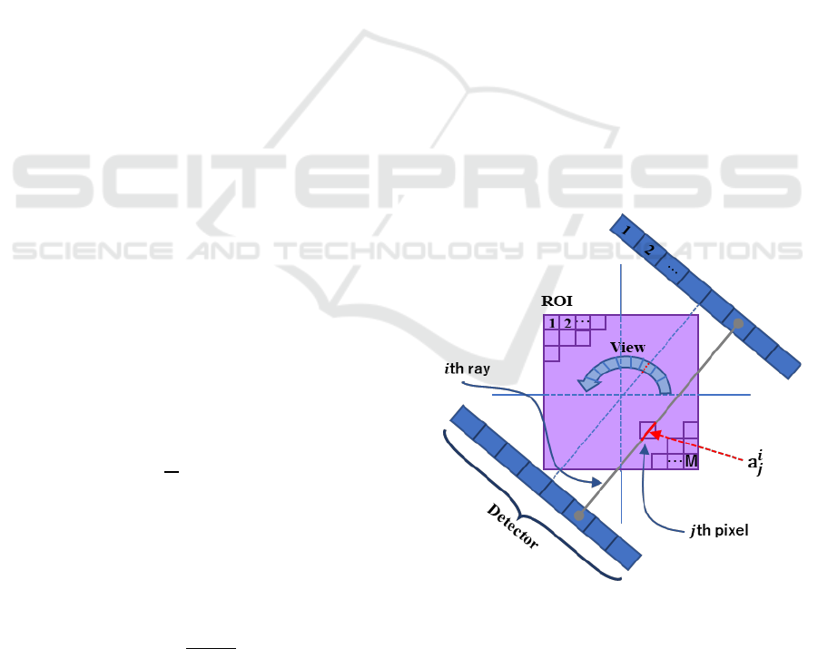
To confirm the effectiveness of the method, computer
simulations were carried out. First, the continuous
object space and the data space are discretized in a
reconstruction problem. A Cartesian grid of the
square observation plane, called pixels, is introduced
into the region of interest (ROI) so that it covers the
whole observation plane that has to be reconstructed
in infinite-dimensional Hilbert space. The pixels are
numbered in some manner. We set the top left corner
pixel 1and bottom right corner pixel M with Raster
scanning.
PHOTOPTICS 2022 - 10th International Conference on Photonics, Optics and Laser Technology
112

Eigenvalue and Eigenvector Expansions for Image Reconstruction
113
where
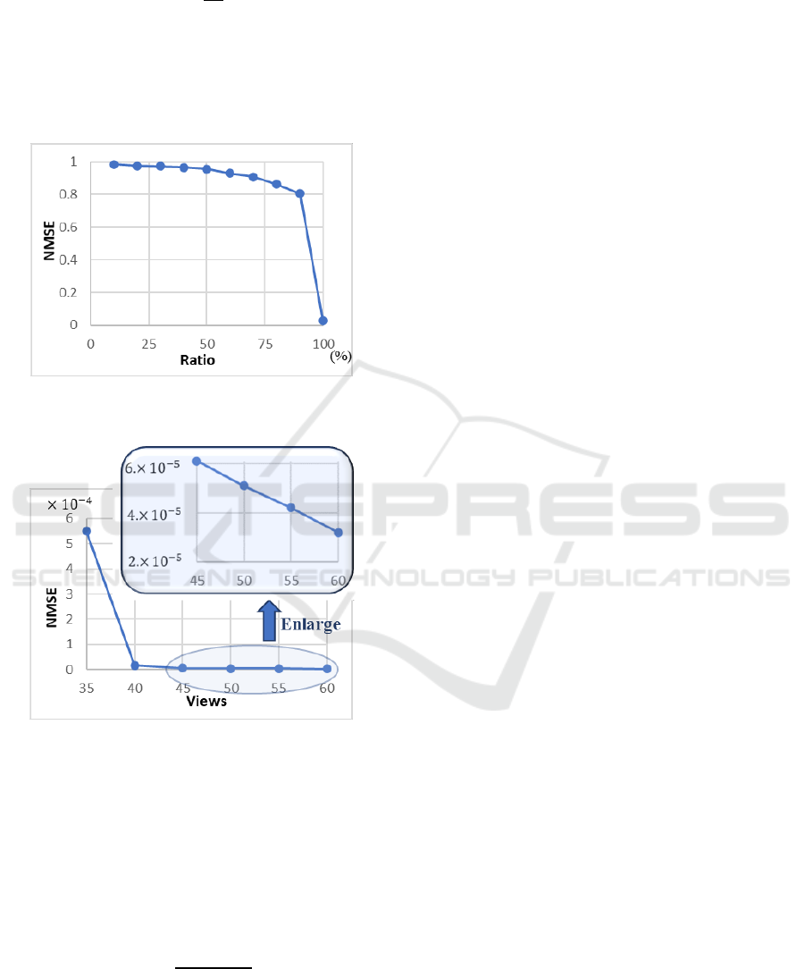
is the image which is reconstructed by
using k eigenvectors and is the original image.
indicates the
-norm. From Fig. 8 we can see that the
error decreases with increasing the number of
eigenvectors.
To check the effect of the number of views in
reconstructed image, we changed the number from 35
to 60. If the number of views is 60 and the number of
detectors per view is 32, the matrix size is
1920×1920. The number of eigenvectors which was
used in reconstruction process is 1024. Figure 9
illustrates the plots of the normalized mean square
error versus the number of views. From Fig. 9 we can
see that the error decreases with increasing the
number of views.
4 CONCLUSIONS
By discretizing the image reconstruction problem, we
applied GARDS to the problem and evaluated the
image quality. In GARDS, it is important
mathematically to reveal the spectrum of bounded
self-adjoint operator in Hilbert space. All eigenvalues
and eigenvectors were computed by Jacobi method.
We showed that the condition number increases with
increasing the number of views. In singular value
decomposition, the condition number play an
important role to solve linear systems. If the condition
number was large, the accuracy of eigen values and
eigen vectors was influenced by the matrix size. Also,
we showed that the error decreases with increasing
the number of eigenvectors and the number of views.
There were many parameters, the number of
views, detectors-source pair and the pixel size of
reconstructed image. The matrix size was changed by
these parameters. If the size was large, computation
of our algorithm consumed time to large quantities.
For a large size of the matrix, especially, it is difficult
to calculate all eigenvalues and eigenvectors with
enough accuracy. The image quality of reconstructed
image in this method is affected by these. If the matrix
size is larger, it is necessary to computer all eigen
values and eigen vectors by the other method, for
example, Lanczos method and so on. Many numerical
methods for large eigen value problems of matrix
have been proposed and reported. It is worth trying to
use these methods. Another idea will be to try to use
parallel matrix computations. These become the
future problems.
REFERENCES
Herman, G. (2009). Fundamentals of Computerized
Tomography, 2
nd
edition, Springer-Verlag London.
PHOTOPTICS 2022 - 10th International Conference on Photonics, Optics and Laser Technology
114

Kak, A., Slaney, M. (1988). Principles of computerized
tomographic imaging, IEEE Press, New York.
Imiya, A. (1985) A direct method of three dimensional
image reconstruction form incomplete projection, Dr.
Thesis, Tokyo Institute of Technology, Tokyo.
[Japanese]
Stark, H. (1987). Image Recovery: theory and application,
Academic Press, New York.
Natterer, F., Wubbeling, F. (2001). Mathematical Methods
in Image Reconstruction, SIAM, Philadelphia.
Bertero, M., Mol, C., Pike, E. (1985). Linear inverse
problems with discrete data. I: general formulation and
singular system analysis, Inverse Problems, 1, 301-330.
Bertero, M., Mol, C., Pike, E. (1988). Linear inverse
problems with discrete data: II. stability and
regularization, Inverse Problems, 4, 573-594.
Andrews, H., Hunt, B. (1977). Digital Image Restoration,
Prentice-Hall, New Jersey.
Ohyama, N., Barrett, H. (1992). A proposal of generalized
analytic reconstruction from discrete samples
(GARDS), Signal Recovery Synthesis IV Technical
Digest, Vol. 11, 105-107.
Yamaya, T., Obi, T., Yamaguchi, M., Ohyama, N. (2000).
An acceleration algorithm for image reconstruction
based on continuous-discrete mapping model. Opt.
Rev., 2, 132-137.
Reed, M., Simon, B. (1972). Methods of Modern
Mathematical Physics. Vol. 1, Academic Press, New
York.
Kuroda, N. (1980). Functional Analysis, Kyoristu
publishing company, Tokyo. [Japanese]
Censor, Y., Elfving, T., Herman, G., Nikazad, T. (2008).
On diagonally-relaxed orthogonal projection methods,
SIAM J. Sci. Comput., 30, 473-504.
Aoyagi, T., Ohstubo, K., Aoyagi, N. (2020). Image
reconstruction by the method of convex projections.
Proceeding of Photoptics 2020, 26-32.
Press, W., Teukolsky, S., Vetterling, W., B. P. Flannery, B.
(1992). Numerical Recipes in C, 2
nd
edition, Cambridge
University Press, Cambridge.
APPENDIX
(18)
Hence, from Eq. (15) and (18), we conclude
(19)
Eigenvalue and Eigenvector Expansions for Image Reconstruction
115
