
Verifiable Executable Models for Decomposable Real-time Systems
Callum M
c
Coll
1 a
, Vladimir Estivill-Castro
2 b
, Morgan M
c
Coll
1 c
and René Hexel
1 d
1
School of Information and Communication Technology, Griffith University, Brisbane, Australia
2
Departament de Tecnologies de la Informació i les Comunicacions, Universitat Pompeu Fabra, Barcelona 08018, Spain
Keywords:
Safety-critical Teal-time Systems, Model-driven Development, Executable Models, Formal Verification.
Abstract:
Formally verifiable, executable models allow the high-level design, implementation, execution, and validation
of reliable systems. But, unbounded complexity, semantic gaps, and combinatorial state explosion have dras-
tically reduced the use of model-driven software engineering for even moderately complex real-time systems.
We introduce a new solution that enables high level, executable models of decomposable real-time systems.
Our novel approach allows verification in both the time domain and the value domain. We show that through
1) the use of a static, worst-case execution time, and 2) our time-triggered deterministic scheduling of arrange-
ments of logic-labelled finite-state machines (LLFSMs), we can create succinct Kripke structures that are fit
for formal verification, including verification of timing properties. We leap further and enable parallel, non-
preemptive scheduling of LLFSMs where verification is feasible as the faithful Kripke structure has bounded
size. We evaluate our approach through a case study where we fully apply a model-driven approach to a hard
time-critical system of parallel sonar sensors.
1 INTRODUCTION
Model-driven software engineering (MDSE) has pro-
gressed remarkably (Bucchiarone et al., 2020; Buc-
chiarone et al., 2021) in creating executable models
that define behaviour at a high level. However, with
the same ease as generating high level behaviours, it
is possible for these to have semantic variants and
thus, formal verification of the model results in cases
where correctness properties hold for some scenar-
ios, but not others (Besnard et al., 2018). This hap-
pens even for a current version of fUML (Guermazi
et al., 2015). Another anomaly with executable mod-
els of UML (fUML) is that race conditions, or exe-
cution paths may diverge, depending on the order of
construction, even if the same model editor is used
to construct the executable model, since there still
are some constructs with ambiguous semantics (Pham
et al., 2017; Estivill-Castro 2021).
Despite the advances in testing approaches, such
as test-driven development (Mäkinen and Münch,
2014) and continuous integration (Hilton et al., 2016),
testing only proves the existence of defects, not their
a
https://orcid.org/0000-0002-9373-0875
b
https://orcid.org/0000-0001-7775-0780
c
https://orcid.org/0000-0003-4217-7210
d
https://orcid.org/0000-0002-9668-849X
nonexistence, whereas formal methods (in particular
model checking) can ensure the correctness of the
software. Thus, it would seem natural that executable
models constructed under MDSE should be suitable
for model checking. In Section 2 we provide a new
perspective into the challenges for verification in the
time domain. This analysis not only reviews the state
of the art, but in Section 3 we show why time-domain
verification with an arbitrary scheduler results in large
sets of possible time-points and further state space ex-
plosion. State space explosion is a major inhibitor to
more widely adopted model-checking to verify exe-
cutable models. Although event-driven programming
has been extremely productive for many types of sys-
tems, it is fundamentally a best-effort approach and
it cannot ensure it meets hard deadlines (Lamport,
1984). Formal verification is significantly more fea-
sible for time-triggered systems than for event-driven
systems (Furrer, 2019).
In Section 4 we analyse the advantages of logic-
labelled finite-state machines (LLFSMs) to reduce
state space explosion in the time-domain. For now,
consider LLFSMs as UML state-charts where events
can no longer label transitions but only guards can.
While this seems to be a restriction, LLFSMs re-
main Turing-complete and there is no loss of expres-
sive power. Moreover, we indicate how the machines
182
McColl, C., Estivill-Castro, V., McColl, M. and Hexel, R.
Verifiable Executable Models for Decomposable Real-time Systems.
DOI: 10.5220/0010812200003119
In Proceedings of the 10th International Conference on Model-Driven Engineering and Software Development (MODELSWARD 2022), pages 182-193
ISBN: 978-989-758-550-0; ISSN: 2184-4348
Copyright
c
2022 by SCITEPRESS – Science and Technology Publications, Lda. All rights reserved

can be statically analysed and scheduled in a time-
triggered fashion. As a result, rather than a machine
waiting in a state for an event to trigger a transition
(which leads to all the issues and complications of the
Run-To-Completion (RTC) semantics (Eriksson et al.,
2003; OMG, 2019; Samek, 2008; Drusinsky, 2006;
Selic et al., 1994)), machines are running the activi-
ties in their states when their turn arrives. This sub-
tle change results in a massive reduction of the state-
space for the model checker. Moreover, because we
can perform static analysis and scheduling, we can
not only verify correctness properties in the value-
domain, but also in the time domain. It may seem
surprising that one is willing to trade the ease of de-
velopment of an event-driven approach for the more
elaborate planning of a schedule in the time-triggered
approach. We argue that for embedded systems, the
event-driven approach (akin to the notion of an inter-
rupt, where the handler suspends the current code)
may not be suitable. Take, for example, the com-
munication channels between the programmable real-
time units (PRUs) and the ARM processors of TI’s
BeagleBone-Black (Molloy, 2014). Here, all syn-
chronisation is through polling the status of Boolean
flags. There often are no operating systems for bare-
metal microcontrollers such as the PRUs, not even a
real-time OS. In Section 5 we present a novel time-
triggered alternative to schedule an arrangement so
that the behaviours execute under controlled concur-
rency. Moreover, we show that modelling with LLF-
SMs facilitates the construction of a schedule. A core
contribution is that we show how we formally verify
that this schedule results in a system that meets prop-
erties in the time domain as well as in the value do-
main. Section 6 describes the design of parallel, non-
preemptive scheduling that is also verifiable. Sec-
tion 7 illustrates the approach with a timing-critical
system of parallel sonar sensors before we conclude
in Section 8.
2 VERIFYING TIME
2.1 Verification of Executable Models
Formal verification is paramount when designing
complex systems, particularly in the domain of
safety-critical real-time systems. MDSE has long
been promising (Selic, 2003) to overcome the lim-
itations of traditional programming languages while
rigorously expressing executable concepts (Mellor,
2003). Executable models strive to remove the dan-
ger of human translation error and ensure that the ex-
ecution semantics corresponds to the target system.
However, formal verification of executable models is
not ideal: as system complexity grows, current ap-
proaches quickly reach their limits, as the compo-
sition of a complex system from multiple subsys-
tems results in a combinatorial state explosion (Seshia
et al., 2018). Model checking verifies abstractions as
a workaround to this problem, but the verified model
is only indicative of what actually runs, introducing a
semantic gap.
Formal verification of a model that does not cor-
respond to its implementation is informative, but po-
tentially worthless. The challenge within real-time
systems is that, in addition to correctness in the
value domain, correctness in time is vital. A value-
domain failure means that an incorrect value is pro-
duced while a temporal failure means that a value
is computed outside the intended interval of real-
time (Kopetz, 2011, Page 139). Temporal verification
is hard, as it must consider all timing combinations
of all possible tasks across all potential schedules.
Such combinations result in an unviable state space
explosion, requiring simplifying assumptions in ex-
isting approaches for formal verification, dangerously
widening the semantic gap.
Time must be treated as a first-order quantity
that can be reasoned upon to verify that a sys-
tem will be able to meet its deadlines (Stankovic,
1988). While UML profiles such as MARTE (An-
dré et al., 2007), and specific languages and tools
such as AADL (Feiler et al., 2005) enable require-
ments engineering of real-time systems, the event-
driven nature and the adoption of the RTC semantics
prevails around UML; thus we still have to see ex-
ecutable (Pham et al., 2017) and formally verifiable
models without semantic gaps (Besnard et al., 2018)
or serious restrictions to specific subsets (Zhang et al.,
2017; Berthomieu et al., 2015). Alternatively the RTC
semantics must be simplified significantly (Jin and
Levy, 2002; Kabous and Nebel, 1999). Till August
2020, Papyrus™ (Guermazi et al., 2015) (the most
UML 2 compliant tool), only had an incomplete Moka
prototype for executing UML state charts. Papyrus
Real Time (Papyrus-RT) UML models show discrep-
ancies with their nuXmv simulation (Sahu et al.,
2020), even in the value domain (let alone the time do-
main) and the (non real-time) C/C++ code of Papyrus-
RT requires a runtime system (RTS) and a C/C++
Development Toolkit (CDT) that use non-real time
Linux concurrency features. Thus, MDSE fails to
guarantee time-related correctness properties.
Verifiable Executable Models for Decomposable Real-time Systems
183

2.2 Models of Time
When performing model checking, the system is rep-
resented as a formal model M that corresponds, with-
out semantic gaps, to a transition system known as a
Kripke structure. A model checker verifies whether
the model M meets some specification φ (D’Silva
et al., 2008) by examining the Kripke structure. The
specification is created through the use of specifi-
cation languages, usually some form of temporal
logic (Alur et al., 1993). However, a prevalent con-
cern for the extended impact of MDSE is whether the
technical difficulties of translating models into code
result in errors due to subtleties in meaning (Selic,
2003) and dangerous semantic gaps (Besnard et al.,
2018). The modelling tool must be able to guarantee
that the semantics defined by the model is the same
when the model is implemented (Mellor, 2003).
Finite-state machines are ubiquitous in modelling
the behaviour of software systems, appearing in
prominent systems modelling tools and languages
such as the UML (OMG, 2012), SysML (Friedenthal
et al., 2009), or timed automata (Alur and Dill, 1994).
In these modelling tools, transitions are usually la-
belled with an event e that triggers the transition.
Model checking approaches that follow these event-
triggered semantics typically use an idealised view of
events that puts aside some of the realities of cyber-
physical systems (Lee, 2008). Often, model checking
tools take the view that events occur on a sparse (or
discrete) time base and that no event can occur while
the system is already processing another event (Alur
and Dill, 1994). Most real-time systems are cyber-
physical systems where events can originate from the
environment (which is not in the sphere of control of
the computer system), meaning that events originate
on a dense (or continuous) time base and may orig-
inate while the computer system is processing other
events (Kopetz, 1992). Importantly, the computer sys-
tem must decide on what happens to events that occur
while the computer system is processing other events.
Are they to be placed on a queue to be processed
later? What priority criteria shall be used to order
events on the queue? Is the queue bounded or un-
bounded? How does the computer system process si-
multaneous events? In rare circumstances such as an
event shower, does the computer system drop events?
And if so, does the computer system choose which
events to drop? Even training materials for certifica-
tion on UML are ambiguous.
“Events that are not processed off the pool are gen-
erally dropped. They will need to be resent to the
state machines for them to be considered. The or-
der the events are examined from the pool is not
specified, though the pool is usually considered an
event queue” (Chonoles, 2017).
Model checking approaches using event-triggered
finite-state semantics often leave these issues un-
defined. This can cause the resulting system
to significantly deviate from the semantics of the
model (von der Beeck, 1994).
The only way to discern the timing of event-
triggered systems is to consider all combinations
of temporal effects of all possible events and event
handlers (Kopetz, 1993). The nature of the non-
deterministic scheduling of the system based around
when events arrive requires considering all possible
combinations. That is, the uncontrollability of the or-
der and frequency of environment events results in un-
controllable concurrency of event handlers, challeng-
ing the capability to reason about timely behaviour
for event-triggered systems particularly when design-
ing temporally accurate real-time systems (Lee et al.,
2017; Furrer, 2019).
3 STATE EXPLOSION
A model checker must inspect all possible execu-
tion paths through a program relevant to the prop-
erties tested. For event-triggered systems, accurate
verification should include configuration of all event
queues. However, most verification tools ignore this
issue (Bhaduri and Ramesh, 2004).
When time verification is required, this must also
take into consideration the execution time of tasks. A
worst-case execution time (WCET) analysis is manda-
tory to ensure deadlines will be met under all circum-
stances. However, the WCET can be prohibitively
complex to analyse when composing a complex sys-
tem from a diversity of subsystems. The execution
time of tasks falls within a range [BCET, WCET]
where BCET is equal to the best-case execution time.
Non-deterministic scheduling based on event occur-
rence and ordering introduces a further state explo-
sion, as any event-triggered task may be executed at
any point in time and in any order. Verification must
therefore ensure that timing deadlines will be met for
any chain of events, where each task responding to an
event takes an execution time somewhere between the
BCET and WCET. To verify such a system, each time
point within this range must be considered, as the sys-
tem behaviour may change, depending on the order-
ing of events. When subsystems communicate using
events, the ordering of events becomes important.
Moreover, a subsystem may generate more events,
which must be handled, causing greater delays. Since
the timing of the system may change depending on
MODELSWARD 2022 - 10th International Conference on Model-Driven Engineering and Software Development
184

the ordering of when events happen, all possible event
combinations must be verified they meet all deadlines.
Timed automata attempt to deal with this issue by us-
ing region automata (Alur et al., 1993, p. 18). This
breaks up the range of possible execution times into
sub-ranges which are used to verify properties under
different combinations of time limits. While timed
automata ameliorate this issue, the technique cannot
remove it altogether. Since state space explosion still
remains, the more complex a system becomes, the
more combinations must be verified. Consider a se-
quence of events e
0
→ e
1
→ ... → e
n
. Even when
we know that the processing of an individual event e
i
takes some time t
e
i
such that BCET
e
i
≤ t
e
i
≤ WCET
e
i
and thus the sequence would be handled no later than
∑
n
i=0
WCET
e
i
, what guarantees can we offer regarding
handling event e
i
, for each i? The following lemma
can be verified by induction.
Lemma 1. For all i,
i
∑
j=0
WCET
e
i
−
i
∑
j=0
BCET
e
i
≤
i+1
∑
j=0
WCET
e
i
−
i+1
∑
j=0
BCET
e
i
.
That is, the range of possible time points increases
monotonically with more events. Moreover, the over-
all amount t of processing time for the sequence of
events is therefore t = t
e
0
when processing only one
event e
0
. However, if the order of events is arbitrary,
and event e
i
arrives somewhere during the handling
of the previous i − 1 events, event e
i
waits on a first-in
first-out queue anywhere between
∑
i
j=0
BCET
e
j
and
∑
i
j=0
WCET
e
j
with numerous partitions possible for
the handling of earlier events. From this discussion,
we can see that the amount of clock values that must
be considered by the verification to ensure bounds
on the lag for handling an event increases with the
length of the event sequence. Moreover, even under
the optimistic assumption that the overhead of event
queuing does not prevent determination of the spe-
cific BCET and WCET bounds for each task, the pos-
sibility to trigger subsequent events causes an over-
all multiplicative effect (and thus, combinatorial state
explosion) that quickly will make time verification in-
feasible for most systems.
4 DETERMINISM WITH LLFSMs
In our approach, we will take advantage of the deter-
ministic schedule for Logic-Labelled Finite-State Ma-
chines (LLFSMs) (Estivill-Castro et al., 2012). LLF-
SMs constitute executable models, enabling model-
driven development. Even with a minimal action lan-
guage (with assignment and integers), LLFSMs are
Turing complete. Thus, there are programs for which
some properties are not verifiable. However, we ac-
cept this is analogous to verifying any system that
is implemented using a Turing-complete language.
We leave open the particular language used for state
actions. However, if a detailed semantics is to be
considered, we can choose IMP (Winskel, 1993) for
the action language compatible with model checkers
such as NuSMV and nuXmv. The important aspect is
that LLFSMs have a deterministic semantics, because
they do not label transitions with events.
Rather than an uncontrolled concurrency at the
mercy of events popping out in the environment or
the system itself, LLFSMs offers controlled concur-
rency and a deterministic schedule. An arrangement
of LLFSMs is ordered and represents a system. Each
LLFSM consists of a finite set S of states and starts
with an initial state s
0
. The system starts with the
initial state of the first LLFSM in the arrangement.
Each transition is labelled with some Boolean logic
expression instead of an event. This fundamentally
changes the model of state execution. Each current
state is not sleeping (as is the case with the event-
triggered flavoured versions of finite-state machines)
and is instead, periodically scheduled. Each transition
is a member of an ordered sequence of transitions. For
the current state, the logical conditions on each tran-
sition are therefore evaluated sequentially, in a deter-
ministic order, from the first transition to the last.
All states have sections that may contain source
code. The sections that execute when the current state
is scheduled constintute a ringlet, and are determined
as follows. The OnEntry section of a state is executed
when the LLFSM first transitions to that state. Con-
versely, OnExit is executed when a transition fires, i.e.
the Boolean expression of some outgoing transition
evaluates to true. Alternatively, if no transition fires,
the code in the Internal section gets executed.
A common schedule is to assign the token of exe-
cution in a round-robin fashion (Estivill-Castro et al.,
2012). However, since a LLFSM ringlet may execute
differently for the same current state, ringlets have
variable duration and are executed one after another
resulting again in a large number of time boundary
values to consider by model-checkers. It would ap-
pear that LLFSMs do not resolve the state explosion
alluded before. However, in Section 5 we will show
how to we can utilise the deterministic order of LLF-
SMs execution to obtain timing guarantees.
M
c
Coll et al. showed (M
c
Coll et al., 2017) that
actual practical implementations of executable LLF-
SMs can be obtained using the Swift programming
language. These implementations have demonstrated
the generation of efficient Kripke structures from ex-
ecutable LLFSMs, which can be used for formal ver-
Verifiable Executable Models for Decomposable Real-time Systems
185
ification in the value domain. The size of these
Kripke structures is minimised through a combina-
tion of strict type-checking rules in combination with
functional programming concepts such as referential
transparency and how communication is modelled be-
tween LLFSMs (M
c
Coll et al., 2017). Recall that a
ringlet represents a single execution of a single state
within a single LLFSM. The execution of a single
ringlet can be made atomic (M
c
Coll et al., 2018)
through the use of context snapshots of the external
variables. The external variables represent variables
that are in the sphere of control of the environment,
e.g., representing the value of sensors. Before the
ringlet is executed, a snapshot of the external vari-
ables is taken. The state that is executed (along with
all transition checks) acts on this snapshot. The state
reads and manipulates variables of the snapshot and
then, when the state has finished executing, writes
the snapshot back out to the environment. This over-
comes inconsistencies where the external variables
may change during the execution of a state, as the
state is only ever acting on the snapshot. This also
simplifies the Kripke structure as the execution of the
state becomes atomic. Since the only way that the
LLFSM can communicate with the sensors/actuators
is through the use of the external variables, the only
Kripke States that matter are those that represent the
configuration of the LLFSM before and after (but not
during) the execution of the state.
We take this idea of an atomic ringlet further, by
introducing the notion of decomposing Kripke struc-
tures into smaller individual structures. LLFSMs that
do not communicate are thus able to be verified in-
dependently within the value domain. However, vari-
ations in the timing of a schedule for LLFSMs must
be resolved if we are to achieve the same effect for
time-domain verification.
5 TIME VERIFICATION
We define the WCET of an LLFSM (denoted
WCET
LLFSM
) as the largest WCET of the set of
all possible ringlets of the LLFSM. Conversely, the
BCET of the LLFSM (denoted BCET
LLFSM
) is equal
to the smallest BCET of the set of all possible ringlets
of the LLFSM. Note that since state sections in LLF-
SMs do not have control structures, these values can
be obtained by static analysis.
The time-triggered model of computation parti-
tions and separates large systems into subsystems
through small, stable interfaces (Kopetz, 1998). Im-
portant here is the concept of a temporal fire-
wall (Kopetz and Nossal, 1997) that allows arrest-
ing the effects of timing dependencies at the sub-
system level, effectively limiting the cumulation of
unbounded propagation (Lamport, 1984) of temporal
dependencies and uncertainty. This has led to the con-
cept of a time-triggered architecture that allows limit-
ing complexity by designing distributed components
around strict, temporal interface constraints (Kopetz
and Bauer, 2003).
Using the sequential static schedule of LLFSM
means that the actual execution time of the sched-
ule cycle would, therefore, fall within a range
[BCET
SC
, WCET
SC
]. We eliminate this range by
changing the schedule to now use a time-triggered se-
mantics. To the best of our knowledge, this is the first
case in the literature of time-triggered schedules con-
taining LLFSMs. To this effect, each LLFSM now
executes within its allotted time slot.
Each time slot is large enough to cover the WCET
of the executing LLFSM. The arrangement of LLF-
SMs still gets dispatched in a round-robin fashion,
however, each time slot is triggered at specific points
in time. Since the time slot is large enough to cover
the WCET of the LLFSM, most of the time, each
LLFSM will finish with some laxity. The system will
execute the ringlet of the next machine at the start of
its time slot, effectively fusing the WCET and BCET
to a single value (the slot duration).
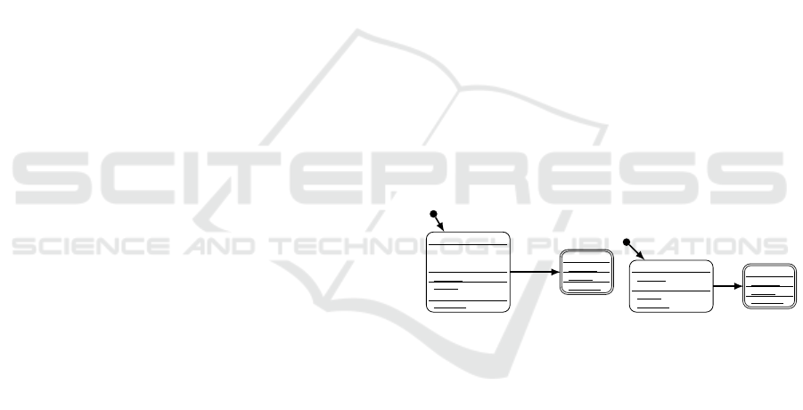
Initial
var a: Int = 2
var b: Int = 3
var result: Int
onEntry
onExit
result = a + b
internal
Terminal
onEntry
onExit
internal
after_ms(20)
(a) The Sum LLFSM.
Initial
onEntry
sleep_ms(30)
onExit
internal
Terminal
onEntry
onExit
internal
true
(b) The Sleeping LLFSM.
Figure 1: Two LLFSMs executing together.
Importantly, the snapshots of the external vari-
ables are taken at the start, immediately upon enter-
ing the time slot and immediately before exiting the
time slot. This effectively reduces the time it takes
for values in the external variables from reaching the
sensors/actuators to a single, deterministic value that
can be measured during WCET analysis. The effects
of this strategy flow onto the timing of the schedule
cycle. Importantly, this makes the timing of every
schedule cycle deterministic and verifiable. Since the
schedule is made up of a few static time slots that
do not change, and we can consider the BCET
SC
and
WCET
SC
equal to the slot duration, the earlier state
explosion disappears. With this approach we then
generate the input for a time transition system (TTS)
which can be evaluated by nuXmv. A TTS in noth-
ing more than a Kripke structure with edges labelled
with durations. nuXmv can represent clocks and ver-
MODELSWARD 2022 - 10th International Conference on Model-Driven Engineering and Software Development
186

ify time-domain properties on the corresponding TTS.
5.1 An Illustrative Example
Considering the LLFSMs shown in Fig. 1 as an ex-
ample. The Sum LLFSM can be reduced to adding
two numbers a and b together and store the sum in
result. However, only after 20 milliseconds, will
the initial state add the numbers together. Since
the computation of the sum is in the OnExit action
of the state, the result value will only be com-
puted just as the system LLFSM transitions to the
Terminal state. The after_ms(20) statement re-
turns a Boolean value indicating whether 20 millisec-
onds have elapsed since the LLFSM first started exe-
cuting the Initial state. The OnEntry action of the
Initial state of the Sleeping LLFSM takes 30 mil-
liseconds to execute. Once it finishes executing the
OnEntry section, it checks its transitions, finds that
the transition marked with true is valid, and will tran-
sition to its Terminal state.
When executing these LLFSMs, we must first
evaluate the WCET of each LLFSM. This will be used
to determine the amount of time allocated to the time
slot for each LLFSM. Let us assume we have anal-
ysed the WCET of the Sum LLFSM to be 5 millisec-
onds. This value would represent the ringlet where
the after_ms(20) transition evaluates to true and the
LLFSM transitions and executes the OnExit action.
For the Sleeping LLFSM, assuming the WCET is 35
milliseconds for instance, captures the ringlet where
the OnEntry action is executed and the system transi-
tions to the Terminal state.
Sum Timeslot
Sleeping Timeslot
|-WCET
Sum
-| |-WCET
Sleeping
-|
Figure 2: The schedule of the two LLFSMs.
Fig. 2 shows how these values result in a static
schedule with two time slots. To perform the verifica-
tion of this schedule, we label the edges of the graph
with time values (Markey and Schnoebelen, 2004).
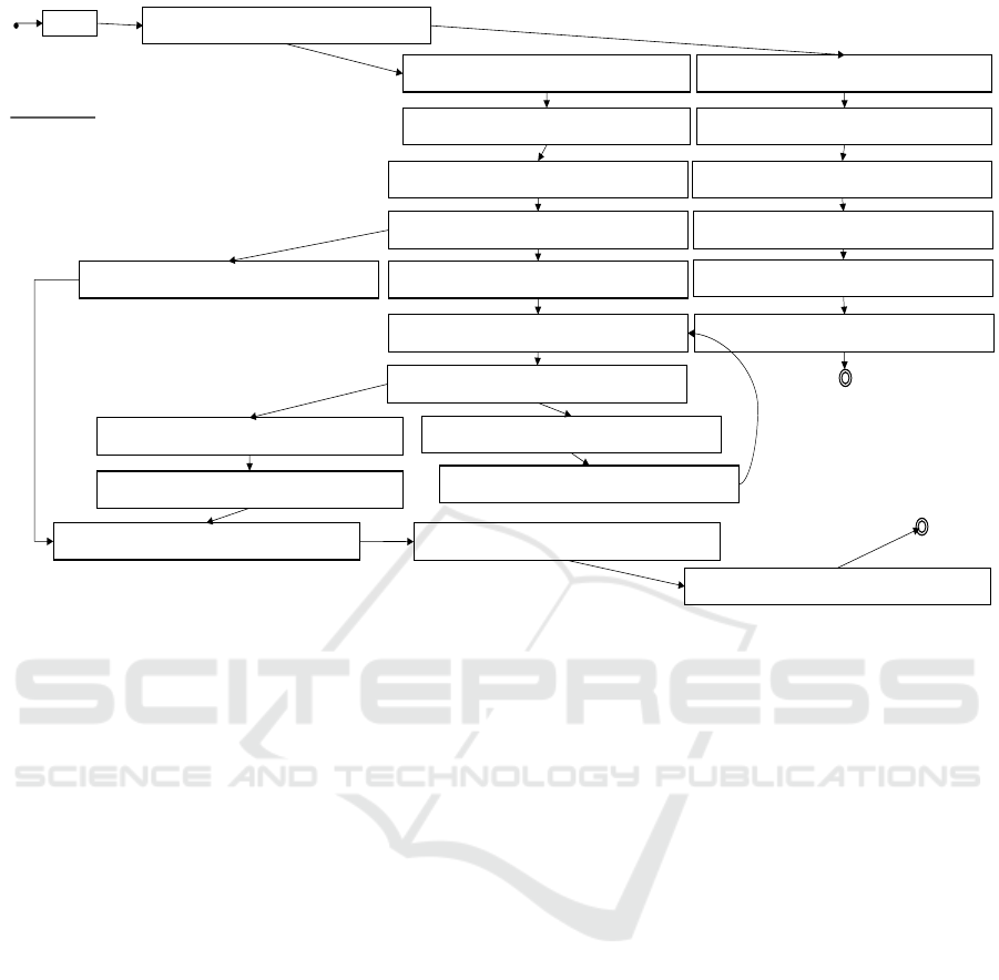
Fig. 3 shows the corresponding Kripke structure.
The resulting Kripke structure demonstrates the
advantage of the time-triggered approach. Each node
contains an evaluation of all variables for all LLFSMs
that have been scheduled, and the program counter
(pc) which indicates which LLFSM is currently exe-
cuting. This program counter is qualified into R (read)
nodes and W (write) nodes. These nodes capture a
snapshot of the external variables, or save the snap-
shot to external output variables, respectively. The
edge between these nodes is labelled with the amount
of time between the reading and writing of the snap-
shots, and is equal to the amount of time allotted to
the time slot. Recall that the activity reads a snapshot
of the external variables immediately upon entering
the time slot and then saves the snapshot immediately
before exiting the time slot. The snapshots are there-
fore read at the start of the time slot and written at the
end of the time slot.
Handling timing transitions (such as
after_ms(20)) is delicate. Taking the example
of the Sum LLFSM, we can see that the configuration
of the LLFSM remains the same until 20 milliseconds
have passed. In other words, this means that only
the clock is changing in the LLFSM. In the Kripke
structure, we deal with this issue by converting the
Kripke structure into a time transition system (TTS)
which can be evaluated by nuXmv. The TTS is made
up of several clocks which are reset at certain points
throughout the graph. The main clock c : R represents
the clock which governs when an edge is available to
be taken. We achieve this with the sync : R variable
that defines the amount of time that must elapse
before transitioning. To this effect, the clock c gets
set to 0, and sync gets set to the amount of time to
wait before transitioning, every time an edge is taken
in the graph.
For example, consider the Sum LLFSM, which
has a time slot of 5 milliseconds. The amount of time
it takes for the system to start executing the LLFSM
within its time slot — represented by the R node —
until the end of the time slot — represented by the
W node — is therefore 5 milliseconds. In the Kripke
structure, the R node thus sets the clock c to 0 and sets
the sync value to 5000, representing 5000 microsec-
onds in this case. The clock c will increase with time
until it reaches the designated 5000 microseconds rep-
resented by the evaluation of sync and causes a tran-
sition to the W node. We use a similar approach to
transition from the W node to the next R node. By util-
ising the c and sync variables, we can create discrete
transition points within the graph which semantically
match the timing of the scheduler when executing the
LLFSMs using time slots.
To handle the a f ter_ms transitions, each LLFSM
within the TTS is also allocated a clock. The clock
for the LLFSM is used to represent the amount of
time that the LLFSM remains within the current state.
The Sum LLFSMs clock c
Sum
here is used to stipu-
late when the LLFSM moves from the Initial state
to the Terminal state. The c
Sum
clock only resets
when the LLFSM transitions to a new state. This
means that as long as the LLFSM remains in the same
state, the c
Sum
clock will continue to increase. The
after_ms(20) transition which limits the LLFSM to
Verifiable Executable Models for Decomposable Real-time Systems
187
pc = initial
SL = {cS = Initial,ringlet = {sEOE = true}}, SM = {cS = Initial,ringlet = {sEOE = true},
states = {Initial = {a = 2,b = 3,result = nil}}}, pc = SM.Initial.R
Abbreviations
SL=Sleeping
SM=Sum
cS=Current State
sEOE = shouldExecuteOnEntry
SL = {cS = Initial,ringlet = {sEOE = true}}, SM = {cS = Initial,ringlet = {sEOE = false},
states = {Initial = {a = 2,b = 3,result = nil}}}, pc = SM.Initial.W
SM.clock := 0
SL = {cS = Initial,ringlet = {sEOE = true}}, SM = {cS = Terminal,ringlet = {sEOE =true},
states = {Initial = {a = 2,b = 3,result = 5}}}, pc = SM.Initial.W
SL = {cS = Initial,ringlet = {sEOE = true}}, SM = {cS = Initial,ringlet = {sEOE = false},
states = {Initial = {a = 2,b = 3,result = nil}}}, pc = SL.Initial.R
SL = {cS = Initial,ringlet = {sEOE = true}}, SM = {cS = Terminal,ringlet = {sEOE =true},
states = {Initial = {a = 2,b = 3,result = 5}}}, pc = SL.Initial.R
5000,SM.clock ≤ 20000
5000,SM.clock > 20000
5000,SL.clock := 0 5000,SL.clock := 0
SL = {cS = Terminal,ringlet = {sEOE = true}}, SM = {cS = Initial,ringlet = {sEOE =false},
states = {Initial = {a = 2,b = 3,result = nil}}}, pc = SL.Initial.W
SL = {cS = Terminal,ringlet = {sEOE=true}}, SM = {cS = Terminal,ringlet = {sEOE=true},
states = {Initial = {a = 2,b = 3,result = 5}}},pc = SL.Initial.W
3500035000
SL = {cS = Terminal,ringlet = {sEOE = true}}, SM = {cS = Initial,ringlet = {sEOE = false},
states = {Initial = {a = 2,b = 3,result = nil}}},pc = SM.Initial.R
SL = {cS = Terminal,ringlet = {sEOE=true}}, SM = {cS = Terminal,ringlet = {sEOE=true},
states = {Initial = {a = 2,b = 3,result = 5}}}, pc = SM.Terminal.R
SM.clock := 0
SL = {cS = Terminal,ringlet = {sEOE = true}}, SM = {cS = Initial,ringlet = {sEOE = false},
states = {Initial = {a = 2,b = 3,result = nil}}}, pc = SM.Initial.W
SL = {cS = Terminal,ringlet = {sEOE=true}}, SM = {cS = Terminal,ringlet= {sEOE=false},
states = {Initial = {a = 2,b = 3,result = 5}}}, pc = SM.Terminal.W
SL = {cS = Terminal,ringlet = {sEOE=true}}, SM = {cS = Terminal,ringlet = {sEOE=true},
states = {Initial = {a = 2,b = 3,result = 5}}},pc = SM.Initial.W
5000
5000,SM.clock > 20000
5000,SM.clock ≤ 20000
SL = {cS = Terminal,ringlet = {sEOE = false}}, SM = {cS = Initial,ringlet = {sEOE = false},
states = {Initial = {a = 2,b = 3,result = nil}}}, pc = SL.Terminal.W
SL = {cS = Terminal,ringlet = {sEOE=false}}, SM={cS = Terminal,ringlet = {sEOE=false},
states = {Initial = {a = 2,b = 3,result = 5}}}, pc = SL.Terminal.W
3500035000
SL = {cS = Terminal,ringlet = {sEOE = false}}, SM = {cS = Initial,ringlet = {sEOE =false},
states = {Initial = {a = 2,b = 3,result = nil}}}, pc = SM.Initial.R
SL = {cS = Terminal,ringlet = {sEOE = false}}, SM = {cS = Initial,ringlet = {sEOE = false},
states = {Initial = {a = 2,b = 3,result = nil}}}, pc = SM.Initial.W
SL = {cS = Terminal,ringlet = {sEOE = false}}, SM = {cS = Initial,ringlet = {sEOE = false},
states = {Initial = {a = 2,b = 3,result = nil}}}, pc = SL.Terminal.R
SL = {cS = Terminal,ringlet = {sEOE=false}}, SM = {cS = Terminal,ringlet = {sEOE=true},
states = {Initial = {a = 2,b = 3,result = 5}}}, pc = SM.Initial.W
SL = {cS = Terminal,ringlet = {sEOE=false}}, SM = {cS = Terminal,ringlet = {sEOE=true},
states = {Initial = {a = 2,b = 3,result = 5}}}, pc = SM.Initial.W
SL = {cS = Terminal,ringlet = {sEOE = false}}, SM = {cS = Terminal,ringlet = {sEOE=true},
states = {Initial = {a = 2,b = 3,result = 5}}}, pc = SL.Terminal.W
5000,SM.clock ≤ 20000
5000,SM.clock > 20000
5000
35000
5000
35000
35000
SL = {cS = Terminal,ringlet = {sEOE =false}}, SM = {cS = Terminal,ringlet = {sEOE=true},
states = {Initial = {a = 2,b = 3,result = 5}}}, pc = SM.Terminal.R
SL = {cS = Terminal,ringlet = {sEOE =false}}, SM = {cS = Terminal,ringlet = {sEOE=false},
states = {Initial = {a = 2,b = 3,result = 5}}}, pc = SM.Terminal.W
SM.clock := 0
5000
Figure 3: Illustration of the entire Kripke structure of the 2-LLFSMs executable model.
transition only after 20 milliseconds can be expressed
in the TTS by creating a guard on the edge leading to
the R node corresponding to the first ringlet when the
LLFSM moves to the Terminal state. The guard is ex-
pressed by an evaluation on the c
Sum
clock with the
usual sync and c guards: c
Sum
> 20000 ∧ c = sync.
Since the LLFSM is not part of a hierarchy and
does therefore not communice, we can apply the opti-
misation discussed earlier and further minimise this
Kripke structure by creating isolated Kripke struc-
tures. These isolated Kripke structures have 5 and 7
nodes respectively. When creating the isolated Kripke
structures, it is important to maintain the timing of
the schedule. Therefore, although the isolated Kripke
structures are able to eliminate nodes of unrelated
LLFSMs, thus avoiding a combinatorial state explo-
sion, they must include the time of the schedule cycle.
This is to account for the timing of all the other LLF-
SMs that are executing, without requiring them to be
included in the Kripke structure.
6 PARALLEL EXECUTION
We now extend our ideas to enable parallel execu-
tion. By utilising a combination of a static sched-
ule and module isolation, we can significantly reduce
and minimise Kripke structures so that scheduling be-
comes deterministic and timing verification becomes
possible. Here we use the same techniques to allow
LLFSMs to execute in parallel.
LLFSMs may exert control over other LLF-
SMs within an LLFSM-hierarchy (Estivill-Castro and
Hexel, 2013a). LLFSMs may also share access to
external variables without concurrency issues. Both
of these features constitute communication lines be-
tween LLFSMs. We leverage the use of an algorithm
that identifies subsystems that can be verified inde-
pendently, and has been utilised for efficient model
checking and failure mode effects analysis (FMEA)
of safety-critical systems (Estivill-Castro and Hexel,
2013b). Here we build on that algorithm to allow par-
titioning of a system into subsystems that can run in
parallel while maintaining verifiability of the system
as a whole in both the time and value domain.
In our earlier example, the Sum and the Sleeping
LLFSMs are not part of a hierarchy and do not use
external variables, thus enabling the creation of iso-
lated Kripke structures. Since these conditions en-
able parallel execution, these two LLFSMs, can exe-
cute simultaneously on at least two cores. The corre-
sponding isolated Kripke structures would reduce the
amount of time between W and R nodes to 0, since the
other LLFSM is executing on a separate core, there
is no wait time. When the dependencies between
all LLFSMs are known, we create a static schedule
MODELSWARD 2022 - 10th International Conference on Model-Driven Engineering and Software Development
188

for each core. We follow (Estivill-Castro and Hexel,
2013b) and create a dependency graph that details the
dependencies that each LLFSM uses to communicate.
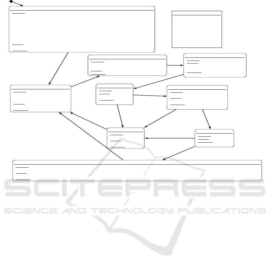
Fig. 4 illustrates this.
We use a dependency graph following Holt’s no-
tation (Holt, 1972). Nodes A, B, C, D and E each
represent an LLFSM. The nodes E
0
and E
1
represent
external variables. The edges of the nodes represent
communication lines. The lines between the LLFSMs
represent the hierarchical owner/slave relationship be-
tween them. Therefore, in Fig. 4, A controls B and
C. The lines connecting the LLFSMs to the external
variables represent LLFSMs that have access to this
particular set of external variables. Importantly, we
extend the semantics of external variables to provide
read-only and write-only semantics. The lines marked
with «read» only read the external variables (sensors).
Any lines marked with «write» (though none appear
in this example) only write to the external variables
(actuators). Those lines that remain unmarked (the
line between A and E
1
for example) follow the orig-
inal semantics where the LLFSMs can both read and
write to the external variables.
This extended semantics facilitates a more fine-
tuned scheduling strategy. In Fig. 4, nodes A and
D can execute at the same time. This is achieved
through a shared snapshot of external variables E
0
.
Since the LLFSMs do not write to the snapshot but
simply read it, they are able to execute their ringlet si-
multaneously, which reads from a shared snapshot of
external variables E
0
. If one of the LLFSMs were to
write to the snapshot, then this would constitute a race
condition. This is why A and E cannot share a snap-
shot of external variable E
1
. Furthermore, we cannot
schedule A, B and C simultaneously as A may exert
control over B and C during the execution. We can,
however, schedule B and C simultaneously since they
are not communicating, and neither are C, D, and E.
Thus, many equivalent schedules are possible.
It is vital that we maintain the use of a static sched-
ule, which allows solving of the NP-hard schedul-
ing problem (Xu and Parnas, 1990) pre-runtime. We
can then verify that the schedule satisfies all con-
straints depicted by the dependency graph before
run-time. Importantly, it has been shown that such
A
B
C
D
E
0
E
1
E
«read»
«read»
«read»
«read»
Figure 4: Example of a dependency graph.
Start Time Length Task Core
0 30 A 1
30 30 C 1
60 40 B 1
0 50 D 2
50 30 E 2
Core 1
Core 2
A
D
C B
E
Figure 5: A possible schedule.
non-preemptive real-time scheduling can be done ef-
ficiently across multi-core processors with shared
caches (Xiao et al., 2017). Fig. 5 shows a possible
configuration of a schedule for a dual-core system.
As depicted in the figure, we can see that the
schedule may contain synchronisation points where
multiple LLFSMs communicate. Recall that A reads
from E
0
but also reads from and writes to E
1
. A
also controls B and C. A is a particularly contentious
LLFSM to schedule as it communicates with many
nodes within the dependency graph. However, we
need to be able to schedule LLFSMs in parallel with
A is executing as to take advantage of the dual-core
system. We can, therefore, execute A and D together.
Once A has finished executing on the first thread, we
can immediately start executing C. Note, that C is
triggered while D is still running on the second thread.
Once D has finished executing, we can also immedi-
ately start executing E on the second thread since E
has no dependencies shared with C. When C has fin-
ished executing, we can then immediately start exe-
cuting B. This may seem to introduce a race condi-
tion. However, since B is writing to the external vari-
ables E
1
after the snapshot is taken by E, it cannot
influence the execution of E. Note that after execut-
ing E, the second thread must wait some time to finish
at the same time as the first thread and thus complete
the scheduled cycle. This resulting laxity is indicated
by the black box after E.
We follow the earlier procedure to create a Kripke
structure. We create 3 isolated Kripke structures:
1. one containing LLFSMs A, B and C,
2. one containing LLFSM D, and
3. one containing LLFSM E.
The cycle time equals the maximum of the cumula-
tive WCETs across cores, and the timed Kripke struc-
ture must account for any laxity on the other cores.
The time between C and B would thus be included in
the transition from the W node of C to the R node of
B. Similarly, for the other Kripke structures, the left-
over time of the schedule cycle labels the transitions
from the W node to the next R node for the D Kripke
structure. For E, the Kripke structure would contain
the execution time of D as well as the laxity at the end
of the schedule.
Verifiable Executable Models for Decomposable Real-time Systems
189

7 THE SONAR CASE STUDY
We will now illustrate, in a realistic case study, the ad-
vantages of our MDSE approach of time-domain ver-
ification of executable models. To this end, we imple-
ment an embedded sonar sensor system that is a vital,
often safety-critical, real-time component in systems
ranging from automotive driver-assist systems to au-
tonomous vehicles and robots.
The model represents a vehicle with several sonar
sensors that measure the distance to potential obsta-
cles. Each sonar sensor covers a section in space
around the vehicle and the sonars are displaced to
prevent propagating signals from interfering. In our
implementation, we use the sonars on a differential
robot to determine the distance to an object. Still, the
notions discussed here are applicable to comparable
sensors that contain emitters and receivers and mea-
sure distance through time-of-flight, e.g. in systems
such as self-driving cars.
The sonar’s operation must record the time it takes
for the signal to travel from the emitter to the object,
and then from the object back to the receiver. The dis-
tance reported is directly proportional to the time, and
its precision and reliance/obsolescence relates to strict
execution timing requirements. Notably, the timing
can vary by orders of magnitude and is in the sphere
of control of the environment (e.g. the changing dis-
tance to an approaching obstacle), rather than the real-
time computer system.
We now show that we can meet strict timing re-
quirements while designing a modular, decomposable
system, i.e. can be composed of individual modules
for each sensor. Moreover, our resulting model will
be scalable, i.e. be able to utilise the module isolation
algorithm from the previous section to avoid combi-
natorial state explosion when generating the corre-
sponding Kripke structure.
While such a state explosion could be avoided if
we implemented this model through a non-preemptive
schedule of measuring tasks, in reality, this is not fea-
sible. Such a solution would cycle through the sonar
sensors by sending out a pulse, waiting for that pulse
to return, calculating the distance, and then executing
a similar task for the subsequent sensor. This is in-
feasible because the act of reading from a sonar sen-
sor involves emitting a pulse and then waiting for that
pulse to return. The further an object is from the sen-
sor, the longer it takes for the pulse to return. Un-
fortunately, this has dire consequences. This is be-
cause it takes an indeterminate amount of time before
the sonar pulse returns (infinity, if there is no obsta-
cle). Even if we bound the time by a maximum dis-
tance, the upper bound for each measurement is or-
ders of magnitude higher than the lower bound when
an obstacle is close. Now imagine a scenario where
task 1 is associated with a clear sensor (i.e. taking its
maximum amount of time). Task 1 is scheduled prior
to task 2 that measures the distance to a rapidly ap-
proaching obstacle. It is easy to envision that the no-
obstacle WCET for Task 1 would cause Task 2 to miss
its deadline resulting in a late sighting.
Switching to a pre-emptive schedule is not scal-
able, as the corresponding models suffer from the
aforementioned combinatorial state explosion. Thus,
we employ our time-triggered approach, which allows
us to create a simple model that will give accurate
readings with deterministic timing and bounded er-
rors. To this end, we have created a system of repli-
cated LLFSMs. Consider the LLFSM depicted in
Fig. 6, operating on a single sonar sensor to produce a
distance calculation. An arrangement of three of these
machines constitutes an executable model that in our
case was then deployed on an Atmel ATmega32U4
Microcontroller, operating at 16MHz, that interfaces
with three external sonar sensors.
In the Setup state, a machine sets up the appropri-
ate pins for reading and writing. Writing to the output
pin in the Skip_Garbage state creates the sonar sig-
nal. The next states are called Wait_For_Pulse_Start,
ClearTrigger and Wait_For_Pulse_End and use the
numloops variable to count the number of ringlets the
machine executes while waiting for the sonar wave to
reflect and register at the input pin. The next states
calculate the distance and transition back to the Setup
states to take a new reading.
Our static schedule calculates the distance by re-
lating time to the number of ringlets executed in our
machine. Since our schedule executes one ringlet in
each machine in turn, the time that the signal travels is
related to the length of the schedule cycle. Since we
have replicated our machines, the WCETs, and thus
the time slots, are of the same length and our sched-
ule cycle is simply 3 × WCET.
In our experiments, the WCET, including dispatch
overhead, was 244µs for each of these machines.
Therefore, the machines time slots are taken from the
following table.
Start Time (µs) Length (µs) Machine
0 244 I
244 244 II
488 244 III
Our overall cycle time is 732µs, which produces a
constant, upper error bound of approximately 13cm.
While this demonstrates that we can achieve a
constant error bound while retaining the ability of
MODELSWARD 2022 - 10th International Conference on Model-Driven Engineering and Software Development
190
Initial
onEntry
triggerPin = 3; echoPin = 2;
distance = 65535; // invalid reading
double NUMBER_OF_MACHINES = 3.0;
SCHEDULE_LENGTH = 0.000244 * NUMBER_OF_MACHINES; // 244 us per machine
SPEED_OF_SOUND = 34300.0; // cm/s
SONAR_OFFSET = 40.0;
uint16_t MAX_DISTANCE = 400;
double MAX_TIME = static_cast<double>(MAX_DISTANCE * 2) / SPEED_OF_SOUND;
maxloops = static_cast<uint16_t>(ceil( MAX_TIME / SCHEDULE_LENGTH));
onExit
numloops = 0;
internal
FSM Variables
uint8_t echoPin;
uint8_t triggerPin;
uint16_t distance;
uint16_t numloops;
uint16_t maxloops;
uint8_t inputPort;
uint8_t inputBit;
double SCHEDULE_LENGTH;
double SPEED_OF_SOUND;
double SONAR_OFFSET;
Setup_Pin
onEntry
pinMode(echoPin, INPUT);
pinMode(triggerPin, OUTPUT);
digitalWrite(triggerPin, LOW);
onExit
digitalWrite(echoPin, LOW);
Internal
SetupMeasure
onEntry
inputBit = digitalPinToBitMask(echoPin);
inputPort = digitalPinToPort(echoPin);
onExit
internal
Skip_Garbage
onEntry
onExit
digitalWrite(triggerPin, HIGH);
++numloops;
internal
++numloops;
Wait_For_Pulse_End
onEntry
onExit
internal
++numloops;
Calculate_Distance
onEntry
distance = static_cast<uint16_t>(max(static_cast<double>(numloops) * SCHEDULE_LENGTH * SPEED_OF_SOUND/2.0 - SONAR_OFFSET, 0.0));
onExit
numloops = 0;
internal
WaitForPulseStart
onEntry
onExit
++numloops;
internal
++numloops;
ClearTrigger
onEntry
digitalWrite(triggerPin, LOW);
onExit
++numloops;
internal
++numloops;
LostPulse
onEntry
distance = 65535;
onExit
numloops = 0;
internal
true
true
true
numloops >= maxloops || (*portInputRegister(inputPort) & inputBit) != inputBit
after_ms(1)
|
numloops >= maxloops
(*portInputRegister(inputPort) & inputBit) == inputBit
--
numloops >= maxloops
numloops >= maxloops
(*portInputRegister(inputPort) & inputBit) != inputBit
\
true
true
Figure 6: The Sonar LLFSM.
model checking in both the value and time domains,
we can further improve this by leveraging our ap-
proach to schedule these LLFSMs in parallel. This is
trivially achievable through module isolation, as the
LLFSMs do not share any dependencies. To this end,
we have created an implementation in the Swift lan-
guage for LLFSMs. This shows that our approach al-
lows not only to utilise a language such as C/C++, but
that it may leverage modern programming languages
such as Swift. Creating an implementation in Swift
provides high-level concepts such as functional pro-
gramming, protocol-oriented design, as well as addi-
tional type safety. Our approach is capable of exe-
cuting not only on just embedded devices, but other
platforms such as desktop or mobile devices.
We use a whiteboard middleware (Estivill-Castro
et al., 2014) to represent sensor input in simulation.
The schedule for the 3 parallel LLFSMs uses a similar
dispatch table, but, the start time of each time slot is 0.
This is because we can leverage a system with at least
three cores, allowing us to schedule these LLFSMs at
the same time. The result of this approach is that the
WCET of the schedule cycle decreases, thus decreas-
ing the amount of error associated with the amount of
time an LLFSM would have to wait before it would be
able to execute its next ringlet. This reduces the error
by a third, since each LLFSM would not have to wait
for other LLFSMs to finish executing their ringlet.
We have generated Kripke structures for both
the sequential and the parallel schedule for the
three sonar machines utilising the swift version of
the Sonar LLFSM. For each variant, 3 separate
isolated Kripke structures were generated each
representing a single sonar LLFSM. In the repository
https://github.com/mipalgu/SonarKripkeStructures
one can find nuXmv source files containing the
Kripke structures as well as graphviz versions which
enable the visualisation of the Kripke structures.
Each of the nuXmv files contains the timed transition
systems for the evaluation of LTL proofs in both
the value and time domains. For example, consider
the proof of Fig. 7, which stipulates that the sonar
machine will always calculate a distance (or fail to
detect any obstacles) within 35 ms.
LTLSPEC
G pc = "Sonar23-Setup_Pin-R" ->
time_until( pc = "Sonar23-LostPulse-W" |
pc = "Sonar23-CalculateDistance-W"
) <= 35000
Figure 7: The LTL Specification For a Guaranteed Result
Delivery Time Interval.
Verifiable Executable Models for Decomposable Real-time Systems
191

8 CONCLUSION
We have demonstrated a MDSE approach for veri-
fiable and executable models of decomposable real-
time systems. We have shown that a time-triggered
model can overcome the combinatorial state explo-
sion and unbounded delays often associated with
event-triggered systems. We can isolate subsystems
to formally verify system execution time bounds, with
the associated ability to handle events within a given
deadline. This has been achieved by creating tem-
poral firewalls between the subsystems involved, us-
ing a static time slot based scheduler. We have fur-
ther demonstrated that this approach can be extended
to parallel, non-preemptive schedules across multi-
ple processor cores. By identifying dependencies be-
tween subsystems, we are able to identify communi-
cation dependencies between the subsystems and cre-
ate fine-tuned schedules.
Our techniques have successfully been applied in
a real-time system case study of vehicular sonar sen-
sors. Through the introduction of the time-triggered
scheduler, we have mitigated the issues that forced
the timing of critical tasks from being tightly coupled
to what is occurring in the environment, i.e. outside
their sphere of control. In doing so, we have shown
how the design of a system can be achieved at a high
level, through an executable model that can be de-
composed into isolated modules, which enables veri-
fication through much smaller Kripke structures, even
when utilising a parallel schedule.
REFERENCES
Alur, R., Courcoubetis, C., and Dill, D. (1993). Model-
checking in dense real-time. Information and Compu-
tation, 104(1):2 – 34.
Alur, R. and Dill, D. (1994). A theory of timed automata.
Theoretical Computer Science, 126(2):183–235.
André, C., Mallet, F., and de Simone, R. (2007). Modeling
time(s). Model Driven Engineering Languages and
Systems, p. 559–573, Springer Berlin.
Berthomieu, B., Bodeveix, J.-P., Dal-Zilio, S., Filali, M.,
Le Botlan, D., Verdier, G., and Vernadat, F. (2015).
Real-time model checking support for AADL. CoRR,
abs/1503.00493.
Besnard, V., Brun, M., Jouault, F., Teodorov, C., and
Dhaussy, P. (2018). Unified LTL verification and em-
bedded execution of UML models. 21th ACM/IEEE
Int. Conf. on Model Driven Engineering Languages
and Systems, MODELS ’18, p. 112–122, NY, USA.
Bhaduri, P. and Ramesh, S. (2004). Model checking of stat-
echart models: Survey and research directions.
Bucchiarone, A., Cabot, J., Paige, R. F., and Pierantonio, A.
(2020). Grand challenges in model-driven engineer-
ing: an analysis of the state of the research. Software
and Systems Modeling, 19(1):5–13.
Bucchiarone, A., Ciccozzi, F., Lambers, L., Pierantonio, A.,
Tichy, M., Tisi, M., Wortmann, A., and Zaytsev, V.
(2021). What is the future of modeling? IEEE Soft-
ware, 38(02):119–127.
Chonoles, M. J. (2017). OCUP 2 Certification Guide
Preparing for the OMG Certified UML 2.5 Profes-
sional 2 Foundation Exam. Morgan Kaufmann, Cam-
bridge, MA 02139.
Drusinsky, D. (2006). Modeling and Verification Us-
ing UML Statecharts: A Working Guide to Reactive
System Design, Runtime Monitoring and Execution-
based Model Checking. Newnes.
D’Silva, V., Kroening, D., and Weissenbacher, G. (2008).
A survey of automated techniques for formal software
verification. IEEE Trans. Computer-Aided Design of
Integrated Circuits and Systems, 27(7):1165–1178.
Eriksson, H.-E., Penker, M., Lyons, B., and Fado, D.
(2003). UML 2 Toolkit. Wiley.
Estivill-Castro, V. (2021). Tutorial Activity Diagrams With
Moka And Unsafe Race Conditions YouTube mipalgu
www.youtube.com/watch?v=P1KX2dBjmO8
Estivill-Castro, V. and Hexel, R. (2013a). Arrange-
ments of finite-state machines - semantics, simulation,
and model checking. MODELSWARD, p. 182–189.
SciTePress.
Estivill-Castro, V. and Hexel, R. (2013b). Module isola-
tion for efficient model checking and its application
to FMEA in model-driven engineering. 8th Int. Conf.
on Evaluation of Novel Approaches to Software Engi-
neering, p. 218–225.
Estivill-Castro, V., Hexel, R., and Lusty, C. (2014). High
performance relaying of C++11 objects across pro-
cesses and logic-labeled finite-state machines. Sim-
ulation, Modeling, and Programming for Autonomous
Robots, p. 182–194. Springer.
Estivill-Castro, V., Hexel, R., and Rosenblueth, D. A.
(2012). Failure mode and effects analysis (FMEA)
and model-checking of software for embedded sys-
tems by sequential scheduling of vectors of logic-
labelled finite-state machines. 7th IET Int. Conf. on
System Safety.
Feiler, P. H., Lewis, B., Vestal, S., and Colbert, E. (2005).
An overview of the SAE architecture analysis & de-
sign language (AADL) standard: A basis for model-
based architecture-driven embedded systems engi-
neering. Architecture Description Languages, p. 3–
15, Boston, MA. Springer US.
Friedenthal, S., Moore, A., and Steiner, R. (2009). A Prac-
tical Guide to SysML: The Systems Modeling Lan-
guage. Morgan Kaufmann, CA, USA.
Furrer, F. (2019). Future-Proof Software-Systems: A Sus-
tainable Evolution Strategy. Springer, Berlin.
OMG (2019). Precise semantics of UML state machines
(PSSM). www.omg.org/spec/PSSM/1.0.
Guermazi, S., Tatibouet, J., Cuccuru, A., Seidewitz, E.,
Dhouib, S., and Gérard, S. (2015). Executable mod-
eling with fUML and Alf in Papyrus: Tooling and ex-
periments. 1st Int. Workshop on Executable Modeling
MODELSWARD 2022 - 10th International Conference on Model-Driven Engineering and Software Development
192

co-located with ACM/IEEE 18th Int. Conf. on Model
Driven Engineering Languages and Systems (MOD-
ELS 2015), vol. 1560, p. 3–8. CEUR-WS.org.
Hilton, M., Tunnell, T., Huang, K., Marinov, D., and Dig,
D. (2016). Usage, costs, and benefits of continuous
integration in open-source projects. 31st IEEE/ACM
Int. Conf. on Automated Software Engineering, ASE
2016, p. 426–437, NY, USA.
Holt, R. C. (1972). Some deadlock properties of computer
systems. ACM Computing Surveys, 4(3):179–196.
Jin, D. and Levy, D. C. (2002). An approach to schedu-
lability analysis of UML-based real-time systems de-
sign. 3rd Int. Workshop on Software and Performance,
WOSP ’02, p. 243–250, NY, USA. ACM.
Kabous, L. and Nebel, W. (1999). Modeling hard real time
systems with UML the OOHARTS approach. 2nd Int.
Conf. on The Unified Modeling Language: Beyond the
Standard, UML’99, page 339–355, Berlin, Springer-
Verlag.
Kopetz, H. (1992). Sparse time versus dense time in dis-
tributed real-time systems. 12th Int. Conf. on Dis-
tributed Computing Systems, p. 460–467.
Kopetz, H. (1993). Should responsive systems be event-
triggered or time-triggered? IEEE Trans. Information
and Systems, E76-D(11):1325–1332.
Kopetz, H. (1998). The time-triggered model of compu-
tation. 19th IEEE Real-Time Systems Symposium, p.
168–177.
Kopetz, H. (2011). Real-Time Systems: Design Principles
for Distributed Embedded Applications. Springer, 2nd
edition.
Kopetz, H. and Bauer, G. (2003). The time-triggered archi-
tecture. Proc. of the IEEE, 91(1):112–126.
Kopetz, H. and Nossal, R. (1997). Temporal firewalls in
large distributed real-time systems. 6th IEEE Com-
puter Society Workshop on Future Trends of Dis-
tributed Computing Systems, p. 310–315.
Lamport, L. (1984). Using time instead of timeout for fault-
tolerant distributed systems. ACM Trans. Program-
ming Languages and Systems, 6:254–280.
Lee, E., Reineke, J., and Zimmer, M. (2017). Abstract
PRET machines. 2017 IEEE Real-Time Systems Sym-
posium, p. 1–11.
Lee, E. A. (2008). Cyber physical systems: Design chal-
lenges. 2008 11th IEEE Int. Symp. on Object and
Component-Oriented Real-Time Distributed Comput-
ing (ISORC), p. 363–369.
Mäkinen, S. and Münch, J. (2014). Effects of test-driven de-
velopment: A comparative analysis of empirical stud-
ies. Software Quality. Model-Based Approaches for
Advanced Software and Systems Engineering, p. 155–
169, Cham. Springer.
Markey, N. and Schnoebelen, P. (2004). Symbolic model
checking for simply-timed systems. Formal Tech-
niques, Modelling and Analysis of Timed and Fault-
Tolerant Systems, p. 102–117, Berlin, Springer.
Mellor, S. J. (2003). Executable and translatable UML. Em-
bedded Systems Programming, 16(2):25–30.
Molloy, D. (2014). Exploring BeagleBone: Tools and Tech-
niques for Building with Embedded Linux. Wiley.
M
c
Coll, C., Estivill-Castro, V., and Hexel, R. (2017). An
OO and functional framework for versatile semantics
of logic-labelled finite state machines. 12th Int. Conf.
on Software Engineering Advances, p. 238–243.
M
c
Coll, C., Estivill-Castro, V., and Hexel, R. (2018). Versa-
tile but precise semantics for logic-labelled finite state
machines. Int. J. on Advances in Software, 11(3 &
4):227–238.
Pham, V. C., Radermacher, A., Gérard, S., and Li, S.
(2017). Complete code generation from UML state
machine. 5th Int. Conf. on Model-Driven Engineering
and Software Development, MODELSWARD 2017,
Porto, Portugal, 2017, p. 208–219. SciTePress.
Sahu, S., Schorr, R., Medina-Bulo, I., and Wagner, M. F.
(2020). Model translation from Papyrus-RT into the
nuXmv model checker. Software Engineering and
Formal Methods. SEFM 2020 Collocated Workshops
- ASYDE, CIFMA, and CoSim-CPS, volume 12524 of
LNCS, p. 3–20. Springer.
Samek, M. (2008). Practical UML Statecharts in C/C++,
Second Edition: Event-Driven Programming for Em-
bedded Systems. Newnes, Newton, MA, USA.
Selic, B. (2003). The pragmatics of model-driven develop-
ment. IEEE Software, 20(5):19–25.
Selic, B., Gullekson, G., and Ward, P. T. (1994). Real-Time
Object-Oriented Modeling. John Wiley, USA.
Seshia, S. A., Sharygina, N., and Tripakis, S. (2018). Mod-
eling for verification. Handbook of Model Checking.,
p. 75–105. Springer.
Stankovic, J. A. (1988). Misconceptions about real-time
computing: a serious problem for next-generation sys-
tems. Computer, 21(10):10–19.
OMG (2012). Information technology - Object Man-
agement Group Unified Modeling Language (OMG
UML), Infrastructure. ISO/IEC 19505-1:2012(E).
ISO.
von der Beeck, M. (1994). A comparison of statecharts
variants. Formal Techniques in Real-Time and Fault-
Tolerant Systems, p. 128–148, Berlin. Springer.
Winskel, G. (1993). The Formal Semantics of Programming
Languages: An Introduction. MIT Press, USA.
Xiao, J., Altmeyer, S., and Pimentel, A. (2017). Schedu-
lability analysis of non-preemptive real-time schedul-
ing for multicore processors with shared caches. IEEE
Real-Time Systems Symposium, p. 199–208.
Xu, J. and Parnas, D. L. (1990). Scheduling processes
with release times, deadlines, precedence and exclu-
sion relations. IEEE Trans. on Software Engineering,
16(3):360–369.
Zhang, F., Zhao, Y., Ma, D., and Niu, W. (2017). Formal
verification of behavioral AADL models by stateful
timed CSP. IEEE Access, 5:27421–27438.
Verifiable Executable Models for Decomposable Real-time Systems
193
