Performance Analysis for Threshold-based N-Systems with

Heterogeneous Servers

Le Anh Thu

1 a

and Tuan Phung-Duc

2 b

Public Policy Program, VNU Vietnam Japan University, My Dinh Campus, Nam Tu Liem, Hanoi,Vietnam

Department of Policy and Planning Sciences, Faculty of Engineering, Information and Systems, University of Tsukuba,

1-1-1 Tennodai, Tsukuba, Ibaraki 305-8573, Japan

Keywords:

Multi-skilled Servers, Threshold Policy, Matrix Analytic Method, Administrative Services.

Abstract:

Driven by the need to develop methods for minimizing operational delays at public administration agencies,

this paper considers problems involving routing and stafﬁng in these agencies. We examine a threshold-based

N-System of two queues with capacities C

= ∞ and C

< ∞, respectively. We use the matrix analytic method

to obtain the steady-state probabilities, the performance measures, and the optimal threshold values in terms

of the system parameters. Our numerical experiments reveal that the mean response time is sensitive to the

stability condition, and the effectiveness of the threshold policy depends on the customer arrival rate.

1 INTRODUCTION

Almost everyone has waited for days or weeks to get

an identity card, a driver’s license, a visitor visa, a

business registration certiﬁcate, etc. Waiting lines or

queues are known as common phenomena in admin-

istrative services due to the inadequate resources in

public administrations and rising demand for these

services, typically in Immigration Department, Busi-

ness Registration Ofﬁce, etc. Queues exist mainly due

to the limited resources of the system. Customer ar-

rivals cannot be scheduled or controlled since the cus-

tomers usually arrive randomly. Moreover, customer

service times are independent random variables; some

individuals take a short time, while others require a

long period. It can be seen that queueing phenom-

ena lead to three common problems: (i) Customer

satisfaction declines due to the discomfort of spend-

ing hours in a crowded waiting room to access the

services; (ii) The employees endure the overloaded

work stress, which reduces the efﬁciency and quality

of work; (iii) Worsening relationships between cus-

tomers and staff, and leading to more disputes.

Waiting time has been identiﬁed as the critical

factor inﬂuencing customer satisfaction, and conse-

quently, decreasing delays has become a focus in op-

timizing the efﬁciency of public services (Osborne

https://orcid.org/0000-0002-1474-134X

https://orcid.org/0000-0002-5002-4946

et al., 2013). Allocating human resources based on

staff capacity is an effective solution for optimizing

staff performance and, as a result, reducing waiting

time. The complexity of work in administrative ser-

vices varies, and so do the qualiﬁcations of the staff.

Experienced employees are advantageous in terms of

performance in highly complex jobs; however, their

performance tends to decline quickly in non-complex

tasks when they become bored. Meanwhile, inexpe-

rienced employees are under pressure as their skills

are not well-matched to their job duties (Hunter and

Thatcher, 2007).

Motivated by these situations, we consider an N-

design multi-server queueing system that serves two

types of customers in two queues. This system em-

ploys two groups of servers: employees trained to

handle low complexity tasks and more experienced

employees who can handle all tasks. The switching

policy of the model is based on the skills of two dif-

ferent types of employees and the thresholds of two

queues. Similar conﬁgurations are found in various

settings, including international call centers (single-

language and multilingual servers), emergency med-

ical departments (life-threatening injuries and oth-

ers), etc. The problem of optimal allocation of cus-

tomers between queues in queueing systems to mini-

mize waiting time has received much attention. As for

the routing and stafﬁng issues, we refer to the survey

paper by Gans et al. (2003).

The model used in this paper is related to the

Thu, L. and Phung-Duc, T.

Performance Analysis for Threshold-based N-Systems with Heterogeneous Servers.

DOI: 10.5220/0010812800003117

In Proceedings of the 11th International Conference on Operations Research and Enterprise Systems (ICORES 2022), pages 137-144

ISBN: 978-989-758-548-7; ISSN: 2184-4372

137

stochastic service systems belonging to a class of

models named ”lane section” that was ﬁrst pro-

posed by Schwartz (1974). Stanford and Grassmann

(1993) considered a similar model of N-design bilin-

gual server system with both specialized and ﬂexible

servers. They presented an exact performance anal-

ysis to determine the minimum number of bilingual

servers required. Due to the computational complex-

ity of this method, only comparatively small systems

can be solved. A closely related model is the paper

by Li and Yue (2016). The authors examined the N-

design call center with two types of users in which pri-

mary users have non-preemptive priority. The state-

space division method has been employed to divide

an inﬁnite number of system states into several ﬁnite

states and obtain the steady-state probability equation

of the system. Shumsky (2004) presented an approx-

imate analysis of a queueing model of the multi-skill

call center in N-design, which has a ﬁxed priority

strategy. The approximate analysis provides reason-

able accuracy while reducing the computational bur-

den of large service centers.

A matrix analytic method has been successfully

applied to the entire state space to obtain exact perfor-

mance measures. Morozov et al. (2021) examined a

modiﬁed Erlang loss system with two classes of cus-

tomers, in which the primary users take precedence

over secondary users. The authors assumed that the

probability distribution of service time is the expo-

nential distribution, then studied the model in depth

by matrix analysis method to evaluate the inﬂuence

of the input parameters on the secondary user perfor-

mance. Perel and Yechiali (2017) studied a closely

related system consisting of two non-identical M/M/1

queues controlled by a threshold-based switching pol-

icy. Jolles et al. (2018) expanded the model of Perel

and Yechiali by adding a switchover time policy.

In order to ﬁnd the mean number of customers in

each queue, the authors formulated the system as a

Quasi-Birth-and-Death (QBD) process. Similar to

the method in Latouche and Ramaswami (1999), they

studied the steady-state behavior of the system and

obtained the rate matrix by applying the matrix ana-

lytic method.

In this paper, we consider the stafﬁng problem of

the N-design model using the matrix-analytic method.

Though queueing analysis has been used in public ser-

vices, this is the ﬁrst analytical result for public ad-

ministration service models with multiple servers in

N-design. The matrix-analytic method allows us to

derive the stability condition and effects of the input

parameters on the mean response time and users’ per-

formance. The advantage of this method is to pro-

vide systematically speciﬁc calculation formulas to

analyze more complicated models while not requir-

ing complex data. Therefore, our model is suitable

for providing evidence to evaluate administrative ser-

vice performance and compare alternatives quickly.

The rest of the paper is structured as follows. In

Section 2, we describe our model with a focus on the

switching policy, while in Section 3, the matrix an-

alytic method is applied to derive performance mea-

sures of the system in steady-state. In Section 4, we

present the results of numerical experiments to show

insights into the performance of our system and vari-

ous phenomena that occur due to a result of changes

in parameters. Section 5 concludes the paper.

2 MODEL DESCRIPTION

We consider an N-design system that serves two

classes of customers with c

and c

servers, respec-

tively. The arrival processes are assumed to be the

Poisson processes with arrival rates λ

and λ

, respec-

tively, and the servers have exponential distributions

with mean 1/µ

for class-i customers, i = 1,2. The

server’s switching policy is threshold-based.

We assume that number of customers in Queue 1

) is not limited while Queue 2 (Q

) can accom-

modate up to N

max

< ∞ customers including the ones

in service. Let C

denote the capacity (the maximum

number of customers accommodated in the system) of

, i = 1,2. We then have C

= ∞, and C

= N

max

< ∞.

If the two capacities C

and C

are inﬁnite, a com-

pletely different approach is required to solve this

problem. For Q

, the threshold level is K ≥ c

, while

for Q

, it is N, c

≤ N ≤ N

max

. Denote by Q

(t) the

number of customers in Q

, i = 1, 2 at time t.

If a customer arrives at Q

and sees this queue al-

ready has N customers, this customer will transfer to

. At that time, if Q

already has K customers, Q

will not accept customers from Q

, and that customer

will return to Q

. The system is illustrated in Figure

Figure 1: The N-design multi-server queueing system.

ICORES 2022 - 11th International Conference on Operations Research and Enterprise Systems

138

3 THE QBD PROCESS

In this section, we calculate the stationary distri-

bution of the Markov process to obtain the cor-

responding stationary performance measures. The

two-dimensional process {(Q

(t),Q

(t)),t ≥ 0} is a

continuous-time Markov Chain with the state space

S given by S = {(i, j) ∈ N × {0,1, .. ., N

max

}}. The

system can be formulated as a Quasi-Birth-and-Death

process (QBD) with the inﬁnitesimal generator Q

given as

Q =







C 0 0 0 ·· · ·· · ·· · ·· · ·· · ··· ·· ·

C 0 0 ···

0 A

C 0 ·· ·

0 ·· · 0 A

C 0 ·· ·

0 0 .. . ... 0 A

K−1

C 0 ...

0 0 .. . ... 0 0 A

0 .. .

0 0 ··· ·· · · ·· 0 0 A

0 .. .







where 0 is a (N

max+1

)×(N

max+1

) zero matrix, and A

,C,C

are (N

max+1

)×(N

max+1

) block matrices given







min(i, c

)µ

0 0 0

0 min(i, c

)µ

0 0

0 .. . 0 min (i,c

)µ







for i < c

, and A

= A

for i ≥ c







i,0

0 0 .. . . .. . .. .. . .. . .. . 0

i,1

0 .. . . .. . .. .. . .. . .. . 0

0 2µ

i,2

0 .. . ... . .. . .. . .. 0

0 ... 0 c

i,c

0 .. . .. . .. . 0

0 ... .. . .. . 0 c

i,N−1

0 .. . 0

0 ... .. . .. . 0 0 c

i,N

0 .. . 0

0 ... .. . .. . . .. ... .. . 0 c

i,N

max−1

0 ... .. . .. . . .. ... .. . ... 0 c

i,N

max







for i = 0, 1,2, ...,K − 1, where b

i,n

= − [λ

+ λ

+ min (i;c

)µ

+ min (n;c

)µ







i,0

0 0 .. . . .. .. . 0

i,1

0 .. . . .. .. . 0

0 2µ

i,2

0 .. . ... 0

0 ... 0 c

i,c

.. . 0

0 ... .. . .. . 0 c

i,N

max

−1

0 ... .. . .. . . .. 0 c

i,N

max







Performance Analysis for Threshold-based N-Systems with Heterogeneous Servers

139

for i = K,K + 1,K + 2,... ,B

= B

, where

i,n

= − [λ

+ λ

+ min (i;c

)µ

+ min (n;c

)µ

for n = 0, 1,. ..,N

max

− 1, and

i,N

max

= − [λ

+ min (i;c

)µ

+ min (n;c

)µ

C =







0 0 ... .. . . .. 0

0 λ

0 ... ... . .. 0

. 0 λ

0 ... 0

0 .. . ... 0 λ

+ λ

... 0

0 .. . ... ... ... 0 λ

+ λ







where the diagonal element C(i, i) is given by

C(i, i) = λ

, for i = 0,1, .. .,N − 1,

C(i, i) = λ

+ λ

, for i = N,N + 1,. .. ,N

max







0 0 0

0 λ

0 0

0 . .. 0 λ







Let M = A

+ B

, then

M =







0 0 . . . . .. 0

0 .. . . .. 0

0 2µ

0 .. . 0

0 ... 0 c

...

0 ... .. . .. . 0 c

max







where the diagonal elements of M is given by

= −(min(i, c

)µ

+ λ

), for i = 0,1, .. .,N

max

− 1,

and m

max

= −c

Let π

= (π

M,i

;i = 1, 2,. .. ,N

max

) be the stationary

probability vector of the matrix M, i.e., π

M = 0

and π

e = 1, where e denotes the column vector

of ones, whose dimension is determined upon context.

The stability condition of such a QBD, (see Theorem

1.7.1, Neuts (1994)) can be obtained by the condition

e < π

This stability condition can be transformed as

< c

. (1)

Let π(i,n) = P(Q

(t) = i, Q

(t) = n), for i ∈ N and

n = 0,1, ...,N

max

denote the stationary probability of

the Markov chain.

We deﬁne

(1)

= (π

i,0

,π

i,1

,. .. ,π

i,N

max

), for i = 0,1,2,...,

(2)

= (π

0,n

,π

1,n

,π

2,n

,. ..) , for n = 0,1,2,..., N

max

According to Matrix-analytic-method (Latouche and

Ramaswami (1999); Phung-Duc et al. (2010)), we

have

(1)

= π

(1)

i−K

, i > K, (2)

(1)

= π

(1)

i−1

(i)

, i = K,K − 1, ...,1, (3)

where R is the minimal non-negative solution of

+ RB

+ R

= 0, (4)

and

(i)

= −C(B

+ R

(i+1)

i+1

)

−1

, for i = K − 1,K − 2, ... , 1,

(5)

given that

(K)

= −C(B

+ RA

)

−1

. (6)

Then, π

is the solution of the following equations

(1)



+ R

(1)



= 0,

(1)

I +

K−1

∑

i=1

∏

j=1

( j)

∏

j=1

( j)

(I − R)

−1

e = 1,

(7)

where we use I to denote the (N

max

+ 1) × (N

max

+ 1)

identity matrix. The ﬁrst and the second equation in

(7) represent the boundary equations at level 0, and

the normalization condition, respectively.

Let E[L

] denote the average number of customers in

the system in Q

, i = 1,2. We then obtain the mean

queue length of Q

and Q

as follows

E [L

] =

∞

∑

i=1

(1)

K−1

∑

i=1

(1)

ie +

∞

∑

i=K

(1)

K−1

∑

i=1

(1)

ie +

∞

∑

i=K

(1)

i−K

K−1

∑

i=1

(1)

ie + π

(1)

∞

∑



+ K



K−1

∑

i=1

(1)

ie + π

(1)

∞

∑

Ke + π

(1)

∞

∑

ICORES 2022 - 11th International Conference on Operations Research and Enterprise Systems

140

K−1

∑

i=1

(1)

ie + π

(1)

(I − R)

−1

Ke + π

(1)

∞

∑

j=1

j−1

K−1

∑

i=1

(1)

ie + π

(1)

(I − R)

−1

Ke + π

(1)

R[(I − R)

−1

]

K−1

∑

i=1

(1)

ie + π

(1)

[(I − R)

−1

K + R[(I − R)

−1

]

]e,

(8)

E [L

] =

max

∑

n=0

(2)

K−1

∑

n=0

(1)

+ π

(1)



I + R + R

+ ···



K−1

∑

n=0

(1)

+ π

(1)

(I − R)

−1

f ,

(9)

where f = (0, 1,2, ...,N

max

)

Let E[L] be the total average number of customers in

the system in both queues, then

E[L] = E [L

] + E [L

]. (10)

We obtain the mean number of busy servers, E[S

], in

, i = 1, 2 as follows

E[S

] =

−1

∑

i=1

(1)

ie + c

∞

∑

j=c

(1)

−1

∑

i=1

(1)

ie + c

K−1

∑

j=c

(1)

e + c

∞

∑

(1)

−1

∑

i=1

(1)

ie + c

K−1

∑

j=c

(1)

e + c

∞

∑

(1)

−K

−1

∑

i=1

(1)

ie + c

K−1

∑

j=c

(1)

e + c

(1)

(I − R)

−1

∑

i=1

(1)

ie +

K−1

∑

j=c

(1)

+ π

(1)

(I − R)

−1

(11)

E[S

] =

−1

∑

i=1

(2)

ie + c

max

∑

j=c

(2)

K−1

∑

n=0

(1)

+ π

(1)

(I − R)

−1

(12)

where g is a (N

max

+ 1) × 1 column vector given by

g = (0, 1,2, ...,c

− 1,c

,. .. ,c

)

Denote by E[T

] the throughput of Q

, i = 1,2, that are

E[T

] = E[S

] × µ

−1

∑

i=1

(1)

ie + c

∞

∑

j=c

(1)

< c

∞

∑

i=1

(1)

eµ

= c

, (13)

E[T

] = E[S

] × µ

. (14)

Then the throughput of the system is given by

E[T ] = E[T

] + E[T

]. (15)

Furthermore, due to Little’s law, we obtain the mean

response time E[R

] in Q

, i = 1,2, respectively, as

follows

E[R

] =

E[L

]

E[Ti]

, for i = 1,2. (16)

The mean system response time is given by

E[R] =

E[L]

E[T ]

. (17)

For reference, we compare with a baseline model,

i.e., two parallel queues without the threshold policy.

In the absence of threshold policy (K = 0), our

system becomes a system of an M/M/c

queue and

an M/M/c

max

queue.

According to Medhi (2002), the probability of zero

customers in the system in Q

is calculated by

(1)

−1

∑

n=0

(λ

/µ

)

(λ

/µ

)

!(1 − λ

/(c

))

−1

The condition for the stability of Q

is λ

/(c

) < 1.

The mean number of customers in the system in Q

given by

E[L

] =

1 − ρ





, (18)

where ρ

, and C





(λ

/µ

)

!(1−λ

/(c

))

(1)

is referred to as Erlang’s C formula.

Then, the mean response time in Q

can be obtained

E[R

] =

E[L

]

. (19)

According to Shortle et al. (2018), the probability of

zero customers in the system in Q

is given by

(2)





−1

∑

n=0





max

− c

+ 1)





−1

for

= 1, and

Performance Analysis for Threshold-based N-Systems with Heterogeneous Servers

141

(2)

−1

∑

n=0





1−





max

−c

1−

−1

for

6= 1, where ρ

Denote by P

max

the blocking probability of Q

which

means that Q

can satisfy atmost N

max

ﬂow units, then

max

(2)

max

−c

The mean number of customers in the system in Q

calculated as

E[L

] =

(2)







1 −



1 −





max

−c

−



1 −



max

− c

+ 1)





max

−c

+ ρ

(1 − P

max

(20)

The mean system response time in Q

can be obtained

E[R

] =

E[L

]

(1 − P

max

)

. (21)

We obtain the mean system response time E[R] in the

case without threshold policy as follows

E[R] =

E[L

] + E[L

]

+ λ

(1 − P

max

)

. (22)

4 NUMERICAL INSIGHTS

This section presents several numerical experiments

of the results obtained in Section 3 to ﬁnd insights

into the performance of our system. For ﬁxed λ

20, λ

= 30, µ

= 8, µ

= 12, c

= 4, c

= 3, and

max

= 50, we show how the performance measures

change according to the thresholds (K,N). Under the

same settings, we also compute these performance

measures in the case without threshold policy (K = 0)

using the classical M/M/c and M/M/c/m models.

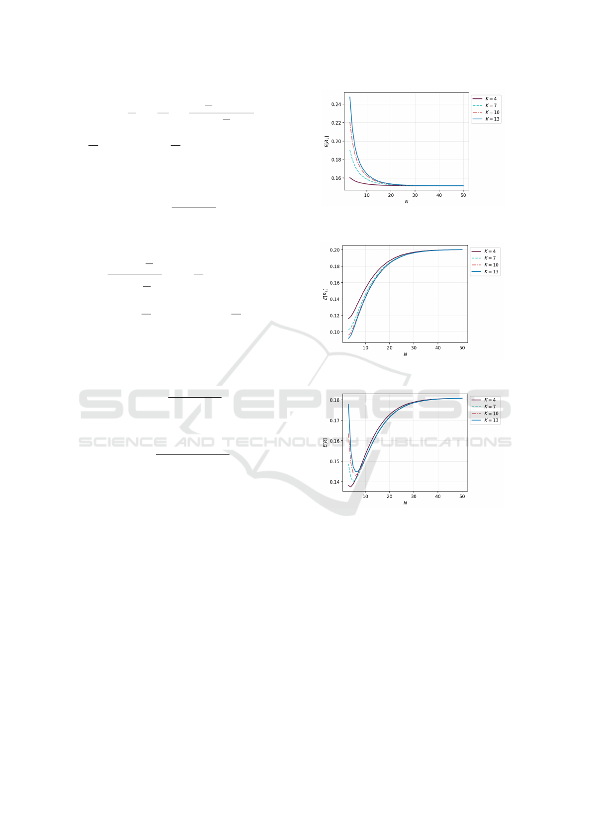
Figure 2 reﬂects the changes in the mean response

time of class-1 customers against Q

’s threshold. The

mean response time of class-1 customers decreases

when N goes up to a speciﬁc value for a ﬁxed K, then

remains unchanged as N continues to increase. Mean-

while, Figure 3 shows the exact opposite trend in the

response time of class-2 customers. It is noticeable

that the mean amount of time that class-2 customers

spend in the system depends more on N than on K.

Figure 2: The mean response time of class-1 customers

against the Q

’s threshold.

Figure 3: The mean response time of class-2 customers

against the Q

’s threshold.

Figure 4: The mean system response time against the Q

’s

threshold.

Figure 4 indicates that the mean system response

time E[R] drops as N goes up to certain thresholds,

then rises again sharply before remaining unchanged

when N is at very high values. For small values of N,

E[R] goes down as N increases and K decreases. This

occurs since the servers in Q

may remain idle even if

there are waiting customers in Q

, including class-2

customers, leading to an increase in the mean system

response time. In this experiment, E[R] reaches the

minimum at 0.1374 when the value of N is 4, and K

is 4. Moreover, the mean response time of the system

without threshold policy is 0.1808, which is higher

than it is in the case of the optimal threshold policy.

For ﬁxed K = 4 and N = 3,9, we show the changes

in the performance measure E[R] against λ

and λ

ICORES 2022 - 11th International Conference on Operations Research and Enterprise Systems

142

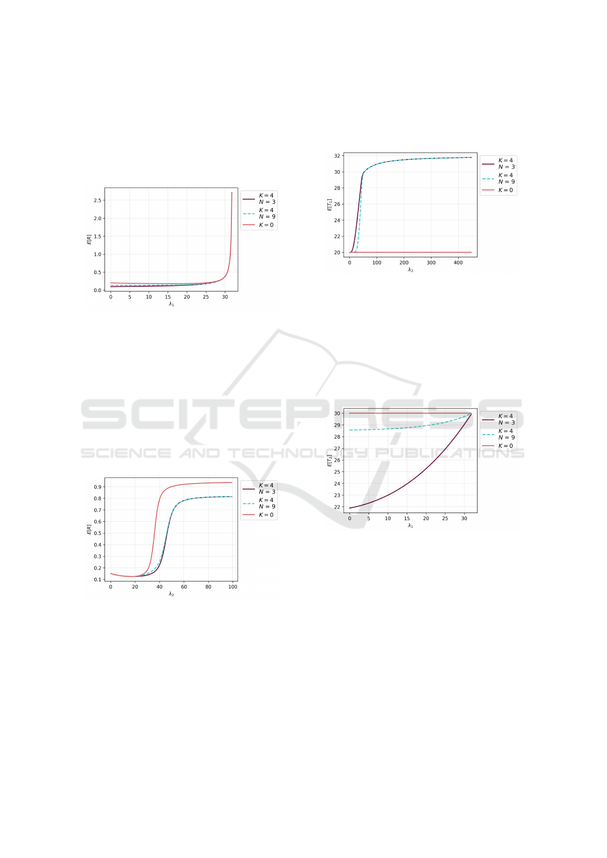
while all other parameters remain unchanged. We

also illustrate the changes in these performance mea-

sures against λ

and λ

in the absence of threshold

policy, thereby ﬁnding that a non-threshold policy is

not optimal for our system. We recall that the stability

condition in both cases with and without the threshold

policy is given by λ

< c

= 32.

Figure 5: The mean system response time E[R] against the

arrival rate of class-1 customers (λ

= 30).

Figure 5 illustrates how the mean system response

time E[R] changes according to the arrival rate of

class-1 customers. The mean system response time is

large when class-1 customers arrive more frequently,

especially as λ

is asymptotic to the value c

. The

mean system response time is highly sensitive to these

values of λ

, while changes in N and K at that time

have no signiﬁcant effect on E[R]. Therefore, as the

arrival rate of class-1 customers approaches the stable

threshold, increasing the number of servers in Q

required to reduce the mean system response time.

Figure 6: The mean system response time E[R] against ar-

rival rate of class-2 customers (λ

= 20).

Figure 6 shows the changes in the mean system

response time E[R] against λ

in both cases with and

without the threshold policy. The performance mea-

sure E[R] in these two cases shares the same trend

when λ

changes. It can be seen that applying the

threshold policy signiﬁcantly reduces the mean sys-

tem response time as the arrival rate of class-2 cus-

tomers is large enough. If class-2 customers arrive

more frequently, the mean system response time is

large, especially within a speciﬁc range of values of

. However, when λ

reaches a certain threshold,

the mean system response time E[R] will stop grow-

ing because the capacity of Q

is limited to N

max

Figure 7: Throughput of Q

against arrival rate of class-2

customers (λ

= 20).

Figure 7 indicates the impact of the arrival rate

of class-2 customers on the throughput of Q

. In the

case of the threshold policy, the throughput E[T

] re-

mains unchanged at λ

when λ

goes up to certain

thresholds, then rises sharply as λ

continues to in-

crease before remains stable at a value of c

(see

the condition (13)) when class-2 customers arrive at

very high rates.

Figure 8: Throughput of Q

against arrival rate of class-1

customers (λ

= 30).

Figure 8 reﬂects the changes in the throughput of

against λ

when λ

is ﬁxed. Under the threshold

policy, the throughput of Q

closely approaches the

value of λ

when λ

is asymptotic to the value of c

For large values of N, the throughput of Q

is insen-

sitive to the arrival rate of class-1 customers. Obvi-

ously, with the threshold policy, the throughput of Q

is greater than or equal to λ

, whereas the through-

put of Q

is less than or equal to λ

because class-

2 customers can transfer from Q

to Q

. In the ab-

sence of threshold policy, the throughputs E[T

] and

E[T

] equal the arrival rates of class-1 and class-2 cus-

tomers, respectively.

Performance Analysis for Threshold-based N-Systems with Heterogeneous Servers

143

5 CONCLUSIONS

This paper has considered the routing and stafﬁng

problems of an administrative agency in an N-design

model that serves two types of customers. Using the

matrix analytic method, we have derived the steady-

state probabilities and the performance measures. We

then have determined the optimal threshold values ac-

cording to the system parameters. We have found

that the threshold policy is highly effective when the

arrival rate of class-1 customers is low and the ar-

rival rate of class-2 customers is high. When λ

ap-

proaches the critical value satisfying the stability con-

dition or λ

is relatively small, increasing the num-

ber of servers combined with changing the threshold

policy is the solution to reduce the mean system re-

sponse time. As a result, we have provided a ba-

sis for reallocating resources when the customer ar-

rival rate changes. Our ﬁndings could be used in

decision-making, managing resources in administra-

tive services, and related applications. It will be help-

ful to expand the analysis of our model to the case

when both capacities are inﬁnite.

ACKNOWLEDGEMENTS

The research of Tuan Phung-Duc was supported in

part by JSPS KAKENHI Grant Numbers 18K18006,

21K11765.

REFERENCES

Gans, N., Koole, G., and Mandelbaum, A. (2003). Tele-

phone call centers: Tutorial, review, and research

prospects. Manufacturing & Service Operations Man-

agement, 5(2):79–141.

Hunter, L. W. and Thatcher, S. M. (2007). Feeling the heat:

Effects of stress, commitment, and job experience on

job performance. Academy of Management Journal,

50(4):953–968.

Jolles, A., Perel, E., and Yechiali, U. (2018). Alternating

server with non-zero switch-over times and opposite-

queue threshold-based switching policy. Performance

Evaluation, 126:22–38.

Latouche, G. and Ramaswami, V. (1999). Introduction

to matrix analytic methods in stochastic modeling.

SIAM.

Li, C.-Y. and Yue, D.-Q. (2016). The stafﬁng problem of

the n-design multi-skill call center based on queuing

model. In Advances in computer science research, 3rd

International Conference on Wireless Communication

and Sensor Network, volume 44, pages 427–432.

Medhi, J. (2002). Stochastic models in queueing theory.

Elsevier.

Morozov, E. V., Rogozin, S., Nguyen, H., and Phung-Duc,

T. (2021). Modiﬁed erlang loss system for cognitive

wireless networks. arXiv preprint arXiv:2103.03222.

Neuts, M. F. (1994). Matrix-geometric solutions in stochas-

tic models: an algorithmic approach. Courier Corpo-

ration.

Osborne, S. P., Radnor, Z., and Nasi, G. (2013). A new the-

ory for public service management? toward a (public)

service-dominant approach. The American Review of

Public Administration, 43(2):135–158.

Perel, E. and Yechiali, U. (2017). Two-queue polling sys-

tems with switching policy based on the queue that is

not being served. Stochastic Models, 33(3):430–450.

Phung-Duc, T., Masuyama, H., Kasahara, S., and Taka-

hashi, Y. (2010). A simple algorithm for the rate ma-

trices of level-dependent qbd processes. In Proceed-

ings of the 5th international conference on queueing

theory and network applications, pages 46–52.

Schwartz, B. L. (1974). Queuing models with lane selec-

tion: a new class of problems. Operations Research,

22(2):331–339.

Shortle, J. F., Thompson, J. M., Gross, D., and Harris, C. M.

(2018). Fundamentals of queueing theory, volume

399. John Wiley & Sons.

Shumsky, R. A. (2004). Approximation and analysis of a

call center with ﬂexible and specialized servers. OR

Spectrum, 26(3):307–330.

Stanford, D. A. and Grassmann, W. K. (1993). The bilin-

gual server system: A queueing model featuring fully

and partially qualiﬁed servers. INFOR: Information

Systems and Operational Research, 31(4):261–277.

ICORES 2022 - 11th International Conference on Operations Research and Enterprise Systems

144