PREUNN: Protocol Reverse Engineering using Neural Networks

Valentin Kiechle

, Matthias B

orsig

2 a

, Sven Nitzsche

2 b

, Ingmar Baumgart

and J

urgen Becker

AMAI GmbH - AI Experts, Karlsruhe, Germany

FZI Research Center for Information Technology, Karlsruhe, Germany

Institute for Information Processing Technology (ITIV), Karlsruhe Institute of Technology (KIT), Karlsruhe, Germany

Keywords:

Protocol Reverse Engineering, Artiﬁcial Intelligence, Machine Learning, Neural Networks, Fuzzing.

Abstract:

The ability of neural networks to universally approximate any function enables them to learn relationships

between arbitrary kinds of data. This offers great potential in information security topics such as protocol

reverse engineering (PRE), which has seen little usage of neural networks (NNs) so far. In this paper, we

provide a novel approach for implementing PRE with solely NNs, demonstrating a simple yet effective re-

verse engineering of text-based protocols. This approach is modular by design and allows for the exchange

of neural network models at any step with better performing models. The architectures used include a convo-

lutional neural network (CNN), an autoencoder (AE), a generative adversarial net (GAN), a long short-term

memory (LSTM), and a self-organizing map (SOM). All of these models combine for a new protocol reverse

engineering approach. The results show that the widespread application layer protocols HTTP and FTP can

successfully be mimicked by artiﬁcial intelligence, thereby paving the way for use cases such as fuzzing. A

direct comparison to other PRE approaches is not possible due to the black-box nature of neural networks and

represents the main limitation of our work. Our experiments showed that this multi-model approach yield up

to 19% better message clustering, improved context distribution, and proving LSTM to be the best candidate

for generating new messages with up to 67.6% valid HTTP packages and 100% valid FTP packages.

1 INTRODUCTION

In 2012 deep neural networks (DNN) (Krizhevsky

et al., 2012) were introduced, showing great ability in

automated feature extraction for classiﬁcation, which

led to a breakthrough in the ImageNet Large Scale Vi-

sual Recognition Challenge (ILSVRC)

. An increas-

ing number of challenges have been tackled by deep

learning since then. One exception to that trend has

been protocol reverse engineering (PRE), as most of

its progress was published from 2004 to 2013, miss-

ing the modern artiﬁcial intelligence (AI) boom. PRE

is a speciﬁc information security task that attempts to

recreate speciﬁcations about an unknown application

layer protocol from artifacts of its communications.

These inferred speciﬁcations can be used in a variety

of other security-related applications such as fuzzing.

The coverage of bugs and edge cases is generally im-

proved with guiding knowledge about the basic mes-

sage structure and internal state of the protocol.

https://orcid.org/0000-0002-6060-6026

https://orcid.org/0000-0002-3327-6957

http://www.image-net.org/challenges/LSVRC/

The capacity of deep learning to mimic network

protocols using reverse engineering and how to model

such an approach are the core scientiﬁc questions that

drove this project. This ability could enable fuzzing

to better harness future advances of the AI research

community. In our initial literature we selected the

two renowned approaches Prospex (Comparetti et al.,

2009) and Discoverer (Cui et al., 2007) to represent

a large body of ideas and strategies commonly used

in PRE. A novel approach is created based on these

two PRE designs to serve as an orientation for solv-

able neural network tasks and a framework for exper-

imentation. We then deﬁne several metrics and im-

plement the experimentation to come to a successful

conclusion. Our key contributions include the anal-

ysis of how to apply deep learning in a modular and

extendable way to the problems of protocol reverse

engineering, implementing a neural network-based

PRE approach on text-based protocols, and showing a

promising direction of future research. There are also

a few minor contributions of smaller workarounds to

solve problems during the experimentation, like the

convolutional embedding for the LSTMs.

Kiechle, V., Börsig, M., Nitzsche, S., Baumgart, I. and Becker, J.

PREUNN: Protocol Reverse Engineering using Neural Networks.

DOI: 10.5220/0010813500003120

In Proceedings of the 8th International Conference on Information Systems Security and Privacy (ICISSP 2022), pages 345-356

ISBN: 978-989-758-553-1; ISSN: 2184-4356

345

2 BACKGROUND

As we attempt to combine two areas of modern re-

search in this paper, a brief overview of both areas’

theoretical backgrounds is given in this section.

2.1 Protocol Reverse Engineering (PRE)

Communication over the internet and other digital

networks requires standardized protocols to ensure

uniform behavior. These protocols are generally used

in a stack with multiple layers, where each layer has

its speciﬁc tasks and serves as the operational basis

for the layers above. The widely known ISO/OSI-7-

layer model works as the standard guideline for such

a protocol stack (TC97, 1984).

Protocols can be divided into four types: text-

based or binary and stateful or stateless. PRE aims

to learn as much as possible about the speciﬁcations

of an unknown protocol by analyzing the artifacts that

the communication creates. This includes, but is not

limited to, message formats, syntax, grammar, con-

stants and keywords, message types, implicit or ex-

plicit state machines, and more. The taxonomy shown

in Table 1 lists the two possible kinds of artifacts: net-

work trafﬁc messages or system calls inside the binary

of an application that communicates using the target

protocol. The two most commonly inferred properties

are the general message format/syntax and the under-

lying state automaton of a stateful protocol. A suc-

cessfully reverse-engineered protocol allows for fur-

ther analysis of the communication like deep package

inspection (Brook, 2018) and fuzzing (Besic, 2019).

Both can work more effectively if they have the de-

tailed speciﬁcation of the protocol.

Two prominent PRE examples are Prospex (Com-

paretti et al., 2009) and Discoverer (Cui et al., 2007).

They were published in the middle of the major period

for PRE research between 2004 and 2013 (Duchene

et al., 2018; Narayan et al., 2015). From our initial

literature research, we judge both to be good represen-

tations of their respective PRE classes, as mentioned

in Table 1.

Protocol Speciﬁcation Extraction (Prospex).

Prospex is a two-part PRE approach basing its

analysis on both network messages and execution

traces of a binary at runtime to infer the message for-

mat (Wondracek et al., 2008; Caballero et al., 2007)

and state automaton in a second part (Comparetti

et al., 2009). The highly distinctive features selected

for the clustering step are among the core reasons for

the success. They include ﬁle system reactions and

memory analysis by tainting bytes. Therefore, the

similarity between messages is not only computed by

their format, but also by the reaction and response

they create. Next, an acceptor automaton was

designed to identify valid sequences of messages.

This automaton was later reduced using the exbar

algorithm (Lang, 1999). The ﬁnal tool was extended

to be compatible with the fuzzing tool Peach Fuzzer

As a direct result, fuzzing can be improved on stateful

protocols. We learn from Prospex how a separation

of tasks such as the extraction of features, clustering

using an off the shelf method and ﬁnally reverse

engineering are key in PRE.

Discoverer. Discoverer identiﬁes small clusters of

tokens within a message, which are then merged and

reﬁned recursively. For this, it relies on the assump-

tion that protocols use common delimiter symbols to

separate parts of their message format, such as com-

mas, whitespaces, or line breaks. The interdepen-

dence of various ﬁelds (e.g., for addresses/variables)

in the message format and their data type (text or bi-

nary) is then learned by heuristics. We can see the

importance of identifying key features and their inﬂu-

ence on clustering in the Discoverer approach.

2.2 Neural Network Architectures

All the models we use in this paper are types of neu-

ral networks. They consist of layers of interconnected

neurons, where each connection has a value to ad-

just the importance of the connection for the next

layer. These weights are adjusted to minimize an er-

ror function during training, but remain ﬁxed for test-

ing and thereafter. This concept allows for compli-

cated mapping of input data distributions to output

results according to the universal approximation the-

orem (Hornik et al., 1989). As such, neural network

architectures are suitable tools for different data op-

erations such as classiﬁcation, regression, clustering,

and more. In the following paragraphs, we describe

the different architectures used in the experimentation

of Section 4, what problems they are good at solving

and why we considered them for PRE.

Convolutional Neural Network (CNN). CNNs be-

came popular for their performance in image recogni-

tion tasks (Krizhevsky et al., 2012). The layers in this

architecture have a particular property: they are used

in a sliding window method over the input data. Their

weights for each of the sliding window steps remain

the same and can therefore be used to detect small,

http://peachfuzzer.com

ICISSP 2022 - 8th International Conference on Information Systems Security and Privacy

346

Table 1: Taxonomy for classifying PRE approaches by requirements (columns) and by results (rows).

PRE taxonomy requirements and results Only network messages Messages and executable binary at runtime

Inferring message format/grammar Discoverer (Cui et al., 2007) Wondracek (Wondracek et al., 2008)

Inferring state automaton PREUNN Prospex (Comparetti et al., 2009)

ﬁxed patterns. Many such “kernels” exist in paral-

lel to each other in separate “channels” of one layer.

This structure allows individual kernels to approxi-

mate highly descriptive feature ﬁlters, thereby remov-

ing the traditional step of manual feature extraction

from the classiﬁcation task. This architecture is ben-

eﬁcial in any task involving images/pixel maps with

individual features occupying many adjacent pixels.

However, in theory, this concept can be applied to any

form of input data with patterns.

Autoencoder (AE). Autoencoders are neural net-

works designed to achieve dimensionality reduction

for a given input while retaining as much information

as possible. In training, the loss function demands

that the output equals the input as closely as possible.

The architecture itself has a bottleneck in a middle

layer to force the network to compress data but keep

reconstructable information (Hinton and Salakhutdi-

nov, 2006). The middle layer’s size has to balance

the compressing size and keep relevant information

in some unknown encoding. Naturally, this divides

the neural network into two components, namely the

encoder and the decoder part. After the AE has been

trained, the decoder element is removed so that any

input data will be returned in its encoded form only.

Generative Adversarial Network (GAN). GANs

were developed to create a generative model for

learned data distribution. The peculiarity of this ar-

chitecture comes from the use of two competing net-

works (Goodfellow et al., 2014). The ﬁrst, known

as generator, uses random noise as input and tries to

create an image similar to those found in the train-

ing dataset. The second network, known as the dis-

criminator, is given either a true or a fake image ran-

domly and has to learn the distinction between them

by merely classifying true from fake. The error cor-

rection for the generator is based on the classiﬁca-

tion result by the discriminator. This combination of

two networks causes a setup of competitive learning

where each NN tries to outdo the opposing one.

Long Short-Term Memory (LSTM). Recurrent

neural networks (RNNs) describe a type of architec-

ture, where some part of the internal hidden or input

state is recursively put into the network again for the

next time step, thereby allowing the network to ﬁnd

time dependencies inside the data. LSTMs are a kind

of RNNs with a strong ability to ﬁnd sequential de-

pendencies over time while avoiding some common

problems with recurrent error correction (Hochreiter

and Schmidhuber, 1997). For working with text data

(sequential letters), it is common to use a dictionary

or alphabet along with a suitable embedding to con-

dense the information in a medium-sized vector for

each word or letter. The text is transformed into a

matrix of length

text

× length

embedding

Self-organizing Map (SOM). SOMs are architec-

tures with one-dimensional or two-dimensional out-

put maps of neurons that contain the topology of the

data (Kohonen, 1982). This means that data with

similar properties and distribution of features will be

found in the same general area of the output map.

Thereby, clustering is implied. SOMs give each out-

put neuron a score related to the data. The winning

node can be returned for indexing.

3 MAIN APPROACH

This section presents a novel way of looking at the un-

derlying task structure of reverse engineering a pro-

tocol. It is divided into multiple steps that are han-

dled mostly sequentially. The approach is designed to

ﬁt the capabilities of various neural network architec-

tures and provides modularity. This allows for the re-

placement of any model in the system by a better per-

forming one and thereby enabling novel AI designs to

be directly inserted into the process.

3.1 Data Gathering

To train a neural network, a representative dataset is

required. We chose a set of text-based application

layer protocol artifacts as a basis to allow for an easier

result evaluation as we do not have a direct compari-

son with other PRE approaches. The chosen protocols

are HTTP v1.1 and FTP because they are commonly

used, abundantly available and lack encryption. We

use several sources of datasets to cover a broader mix

of implementations and message type distribution.

PREUNN: Protocol Reverse Engineering using Neural Networks

347

3.2 Feature Extraction

In this ﬁrst part, we want to extract highly distinguish-

able features. Both in Prospex and Discoverer, the

feature selection was an essential part of the work,

but the features were chosen by the researchers. We

intend to automate this process with neural networks.

Of particular interest are keywords, punctuation, syn-

tactic characters, and other patterns that distinguish

between different messages. Pseudo-random strings

such as tags and cookies are avoided, as they are gen-

erally unrelated to the protocol speciﬁcations.

3.3 Feature Reverse Engineering

In traditional protocol reverse engineering, the anal-

ysis infers rules, lists of variables or constants, and

grammar from the communication artifacts. With a

neural network, the learned knowledge is intrinsically

non-representative, meaning it is challenging to in-

terpret by humans. We use a generative evaluation

approach to judge the quality of the features learned

(and recreated) by the respective architectures. Such

a method will create new samples from the training

distribution and provide insights into what the neural

networks learned.

3.4 Clustering

Protocol messages can usually be grouped into types

whether or not the protocol explicitly speciﬁed these

groups. We can cluster these messages using infor-

mation like sequential order, functionality and general

format. The clustering would imply various types of

messages, and we consider this task to be well-suited

for neural networks (Bac¸

ao et al., 2005).

3.5 State Recognition

A typical communication session usually involves

multiple messages being sent or received. In stateful

protocols, particular sequences of messages achieve a

more complex state between the communication par-

ties. These sequential patterns imply a representative

state automaton for the inner state of the protocol. We

think that a neural network with the capability of un-

derstanding sequential dependencies should be able

to learn the order of different message types and their

likelihood. This interpretation allows the usage of

time series prediction to imply the next state of the

protocol.

3.6 Sequence Generation

As a last step, we combine all trained models into one

generative PREUNN AI. Context information such as

cluster index and sequential dependencies can be in-

cluded in the feature reverse engineering to achieve

more accurate results. Ideally, this AI is capable of

producing valid messages, which are not part of the

training set but have comparable statistical properties.

4 EXPERIMENTS

This section lists all implementations for the main ap-

proach and the experiments, that were used to test var-

ious neural network architectures. The hyperparame-

ters of all neural networks are set to well-performing

numbers after some semi-extensive manual testing.

The scope of the project did not include major opti-

mizations as the hardware was unable to handle large

search spaces for automated hyperparameter tuning.

Our code is available on GitHub

. All experiments

were written in Python 3 using an object-oriented pro-

gramming style to ensure easy modiﬁcation and ex-

tension of the experiments to new protocols. We se-

lected PyTorch

as the deep learning framework, and

all experiments were conducted on an NVIDIA GTX

970.

4.1 Data Preprocessing

We used two datasets in our tests. The ﬁrst one con-

sists of the combination of multiple HTTP sources

(Garﬁnkel, 2008; Shiravi et al., 2012; Goo et al.,

2019; Sharafaldin et al., 2019) that were selected to

cover different implementations and scenarios. The

second dataset consists of FTP messages (Pang and

Paxson, 2003). Before any experiments can be con-

ducted, we examined the data for outliers and irregu-

larities. Data engineering usually takes up a signiﬁ-

cant amount of time in any machine learning project;

however, with network traces in pcap ﬁles, we were

able to shorten this process. The network analysis tool

Wireshark

provides a widely used parser for proto-

col package analysis. We ﬁltered for valid packages

of HTTP and FTP respectively and discarded the rest.

The length of application layer datagrams is lim-

ited by the underlying TCP protocol. An analysis of

the new pcap ﬁle showed that lengthy messages only

occur at image transfers (HTTP) or custom messages

https://github.com/PREUNN/preunn

https://pytorch.org/

https://www.wireshark.org/

ICISSP 2022 - 8th International Conference on Information Systems Security and Privacy

348

(FTP) and can subsequently be cut without signiﬁcant

loss of information. We chose the length limit of 1024

bytes for all packages to uniform the neural network

inputs. Only 0.33% of HTTP and 0.18% of FTP data

that we use exceed this length limit.

As a further step for the HTTP experiments, all

content after the message header was removed, to

avoid XML and other non-HTTP data. We achieved

this by splitting each statement at every “\r\n\r\n”

occurrence and only using the ﬁrst element of that

split. This double line break is the HTTP sign for

only payload following, and thus represents a conve-

nient way to clean the data. No ﬁlter was applied for

the FTP data.

Dataset bias is a common pitfall when developing

machine learning solutions. It describes an uneven

distribution of classes within the data, which causes

suboptimal feature learning in the neural networks.

The protocols themselves do not specify classes of

messages directly; however, the manually created

classiﬁcation for both protocols are our baselines to

orient the class balance on. It is desirable that the neu-

ral networks still learn which types are more common

than others, but the imbalance in our dataset is over-

whelmingly in favor of two or three common message

types. To balance the number of messages per class,

we came up with this improvised formula:

samples per class

occurrences

∗ 100 (1)

and visualized the distribution to see the effect in ﬁg-

ure 1 and 2.

The packages for each class were selected ran-

domly until the limit was reached. This includes mul-

tiplications of rare messages to get a signiﬁcant sam-

ple size in every class. Tests without this dataset bal-

ancing have shown strong signs of overﬁtting in most

experiments. We did not simply set all classes to the

same limit, as the notion of common and uncommon

should not be lost.

4.2 Feature Extraction

Neural networks are known to be highly ﬂexible self-

learning feature extractors across various tasks. When

we try to interpret each message character as a pixel

integer value and thus the entire message as a one-

dimensional image, we can apply solutions for image-

based tasks. We selected two types of architectures

for feature extraction: an autoencoder and a convolu-

tional neural network. The feature mappings learned

by the models in these experiments later serve as input

to the clustering. By the black-box nature of neural

networks, we cannot directly measure the quality of

the feature mappings and will instead use the later re-

Figure 1: HTTP dataset distributions in original (blue) and

balanced (green). The overwhelming bias in favor of GET

messages has been mitigated while preserving the notion of

this type being the most common.

Figure 2: FTP dataset distributions in original (blue) and

balanced (green). With three dominant types and several

underrepresented types, the rebalancing smoothed the dis-

tribution signiﬁcantly while preserving tendencies.

sults from clustering to evaluate both architecture. We

only deﬁned auxiliary metrics for each experiment.

Autoencoder. Autoencoders only work on data of

ﬁxed length and learn a compact representation of the

data. The network messages we use as data vary in

length, but generally do not exceed 1024 bytes. To

unify them, we pad shorter messages with zeros to

ﬁll up the length of 1024. Small-scale tests indicate,

that padding/capping to this length does not impact

the performance of any model signiﬁcantly. As the

expected output for the AE architecture is equal to

the input, we used the Hamming distance as a guid-

ing measure for success during the experimentation.

We train an autoencoder the following layer sizes:

1024 → 256 → 128 → 256 → 1024. We use softplus

activations, the Adam optimizer is set to a learning

rate = 0.0005, the loss function is Mean Square Er-

PREUNN: Protocol Reverse Engineering using Neural Networks

349

ror (MSE), and the batch size = 128 for 10 epochs.

We use the resulting 128 neurons wide output of the

encoder part as the feature encoding for a message.

The data for this experiment was interpreted as pixels

and subsequently has a continuous nature in the inter-

val [0, 255]. The distance achieved for data samples

of length 1024 bytes in training is 254.44 on average

for HTTP and 41.28 for FTP. The very high Ham-

ming distance results from the continuous nature of

the byte interpretations, even the padding symbols (0)

couldn’t be reconstructed entirely. We observe that

padding symbols often miss the same ASCII symbol

by 1 or 2 values if we interpret the ASCII table as

a scale from 0 to 255. In an image, such small col-

oration mistakes would hardly be noticeable. For the

alphabet as a continuous scale, the results often look

wrong. However, an autoencoder’s primary purpose

is to reduce the feature dimensionality for minimal

loss of information and the learning of patterns. In

this case, we managed to reduce the dimension from

1024 down to 128 while retaining satisfying recon-

struction properties during the experimentation. The

lower average Hamming distance for FTP can be ex-

plained by their much shorter average message length.

Convolutional Neural Network. CNNs are com-

monly used for supervised image classiﬁcation. Our

training data does not contain any labels that can be

used for supervised learning. We came up with our

own unsupervised learning technique using data aug-

mentation. Messages are replicated and modiﬁed into

several known classes of augmentation types to ex-

tract information about the syntactic context. Our idea

is, that the ability of a CNN to differentiate between

these augmentation classes will teach it to become

ﬁne-tuned to common patterns in the syntax. HTTP

or FTP statements are again padded/capped to a ﬁxed

length of 1024, then divided into segments of vari-

ous lengths (1024, 32, 16, 8, 4), which are then put

into random order within the same statement. This ap-

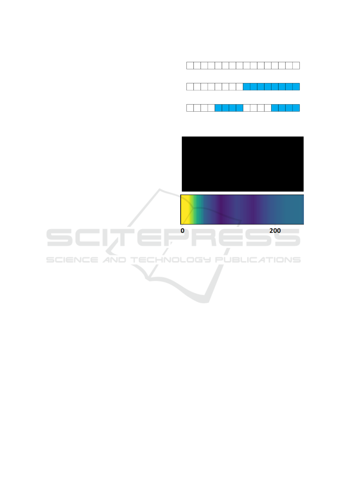
proach results in 5 classes (unchanged and scrambled

into blocks of length 32, 16, 8, and 4, respectively). A

simpliﬁed example is illustrated in ﬁgure 3.

We chose an architecture that uses blocks of 1D

convolution, 1D batch normalization, softplus activa-

tion, and 20%-dropout in a total of 5 layers following

the channel sizes as follows: 1 → 128 → 64 → 32 →

16 → 8. The classiﬁcation task was performed by two

fully connected layers, which were removed after the

training to get a feature map of 8 ∗ 30 = 240 neurons,

which is larger than that of the autoencoder. We used

a visualization of the learned features as an additional

analytical method to evaluate the performance. A va-

riety of methods for model explanation have been pro-

Class 1: unchanged

H T T P

1 2

0 0

Class 2: length of blocks: 8

0 0

H T T P

Class 3: length of blocks: 4

1 2

0 0

H T T P

Figure 3: An HTTP statement scrambled into 3 classes (un-

changed and blocks of length 8 and 4). The color indicates

the block-size and the order of the blocks is randomized.

HTTP/1.1 200 OK

Date: Mon, 14 Jun 2010 11:33:55 GMT

Server: Apache/2.2.3 (Red Hat)

Last-Modified: Mon, 22 Jun 2009 21:03:26 GMT

ETag: "1ef8b2d-59-46cf634892380"

Accept-Ranges: bytes

Content-Length: 89

Vary: User-Agent

Content-Typ: image/gif

Figure 4: Example of HTTP statement classiﬁcation score

visualized by Grad-CAM. The padding has been cut off.

The semantically signiﬁcant and consistent parts are high-

lighted, while pseudo randomness in the ETag is ignored.

The text highlighting in this ﬁgure is an approximation.

posed for image classiﬁcation tasks. We use the vi-

sualization of pixel importance known as Grad-CAM

(Selvaraju et al., 2017) as our quality measurement

for syntactical features found by the model. Our ex-

periments showed mixed results. Regarding HTTP,

we see that various parts of a protocol message are

highlighted differently, see ﬁgure 4. The highlighted

parts often match syntactically relevant pieces, while

pseudo-random strings are ignored. This is precisely

the kind of syntactical feature extraction that is de-

sired for this experiment.

For FTP, the results are less visible in Grad-CAM,

as the average message length is much smaller. The

overall convergence of the experiment was also much

ﬂatter than that of the HTTP version.

4.3 Feature Reverse Engineering

A common result of protocol reverse engineering is

the representation of the target protocol in the form

of rules or clusters. Neural networks do not allow

us to directly visualize their internal representation of

ICISSP 2022 - 8th International Conference on Information Systems Security and Privacy

350

the features they extracted, however. To have a tan-

gible result outside clustering and sequence recogni-

tion, we want to be able to generate new messages as

proof of the correctness of the feature learning abil-

ity. We achieve this by using generative neural net-

work models and examine their outputs. There are

two possible choices of how a text message can be in-

terpreted: an image-like byte interpretation (as in the

feature extraction before) or a sequential interpreta-

tion as a sequence of ASCII alphabet symbols. We in-

vestigated both alternatives, using a default GAN ar-

chitecture for image-like byte interpretation, roughly

following the suggestions given by the original au-

thors (Goodfellow et al., 2014; Radford et al., 2015),

and an LSTM model for interpretation as a sequence

of ASCII symbols, with a modiﬁed embedding for

accounting the randomness in some parts of protocol

messages (cookies, addresses, etc.).

Generative Adversarial Net. The two networks a

GAN consists of, the generator and the discrimina-

tor, are trained in parallel. The generator uses four

1D transposed convolution layers with (kernel size,

stride)-parameter tuples of (2, 2), (4, 4), (8, 8), and

(16, 16) in ascending order. The ﬁrst three layers

are followed by a 1D batch normalization and ReLU

activation each, while the last one ends with a sig-

moid function. The number of channels is as fol-

lows: 1024 → 1024 → 128 → 32 → 1. The dis-

criminator uses four 1D convolution layers with 1D

batch normalization (except for the ﬁrst layer) and

LeakyReLU with a 0.2 slope and 20%-dropout. The

network is capped with a 360-neuron fully connected

layer. Channels are as follows: 1 → 10 → 20 → 60 →

90 → 1. We use a formula to keep either network

from overtaking the other in training: If one network

error went over a threshold OR the other network un-

der a particular border, then the overperforming net-

work is removed from training until the other catches

up. Both use an Adam optimizer with a learning rate

= 0.0005 and betas = (0.5, 0.99). As a loss function,

we used Binary Cross-Entropy (BCE).

The GAN model’s training did not indicate a sig-

niﬁcant convergence towards a stable state. As the

pixel interpretation’s inaccuracy is limiting the GAN

from the start, combined with this architecture’s gen-

erally unstable nature, we are not surprised by this

disappointing result. Creating text from a continu-

ous data interpretation only sounded promising to us

when we considered the static structure used by a pro-

tocol. However, not even the padding symbols have

successfully been replicated with any signiﬁcant ac-

curacy (about ±3 ASCII values) by the GAN model.

Further, experiments using this architecture are omit-

ted.

Long Short-Term Memory. LSTMs are advanced

recurrent networks, trained on sequences of ﬁxed

lengths. To create such conditions, padding is out of

the question, as it would insert undesirable sequential

dependencies. We instead use a script, which con-

catenates statements to achieve more than four times

the required length, then choosing a substring of cor-

rect length starting from a random position. This

script is only used for the training to teach the se-

quential dependencies from letter to letter. Before

and after each statement, a unique symbol for start-

of-package (SOP) and end-of-package (EOP) is in-

serted so that the network can learn to distinguish

between different messages. The data is represented

as a one-hot-encoding of the ASCII alphabet. The

architecture uses an embedding layer followed by a

convolution layer (kernel size=4, stride=4) for em-

bedding adjustment. This trick is introduced here

as convolutional embedding, designed to balance be-

tween character-based and word-based embedding in

data formats with a lot of random noise on character

level. The hidden size of the embedding is ﬂipped

with the feature-length dimension of the tensor; the

convolution layer interprets the hidden width as chan-

nels and the feature-length dimensions as image di-

mensions. Only the batch size remains the same. This

dimension transposition is reversed after the convolu-

tion, resulting in an embedded tensor with a quarter of

the length. This is given as input to a single-layered

LSTM. The output goes through the reversed pro-

cedure of the convolution embedding in a 1D trans-

posed convolution and a fully connected layer with

the same hyperparameters and dimension transposi-

tions. Figure 5 shows an overview of how this em-

bedding works. The way to interpret this kind of em-

bedding is a learnable, weighted 4-gram of charac-

ters, where the whole architecture only has to learn

the next character (from 0–1023 to 1–1024 by index).

This local context inside the 4-gram and the long-term

dependencies, which have been shortened by a factor

of 4, are easier to learn for the model and more sta-

ble to sample. For training, an Adam optimizer with a

learning rate = 0.005 and standard beta is used. Nega-

tive Log-Likelihood (NLL) is used as the loss func-

tion since the error is measured on character level.

This, of course, requires the input data mentioned at

the top to consist of message strings with a length that

are multiples of 4.

This sequence-based attempt at recreating HTTP

and FTP statements shows good results. The LSTM

architecture converges towards a minimal loss after

less than one epoch, indicating excellent structural

PREUNN: Protocol Reverse Engineering using Neural Networks

351

H T T P

1 2

0 0

H T T P

1 2

0 0

O S

H T T P

3 0

E D

...

Batch of sequences

Conv

4:1

Conv

4:1

Conv

4:1

Conv

4:1

Conv

4:1

Batch of 1D images

(ﬂipped tensor dimensions)

Batch of sequences

...

Figure 5: Simpliﬁed illustration of the convolutional em-

bedding. It allows for a weighted length reduction of text

and increases the size of the alphabet.

HTTP/1.1 200 OK

Date: Mon, 14 Jun 2010 13:20:25 GMT

Server: Apache

Last-Modified: Mon, 21 Jun 2010 14:18:09 GMT

ETag: "2de9573-2b-486717fb77ac0"

Accepted-Ranges: bytes

Content-Length: 43

Connection: close

Content-Type: text/html; charset=iso-8859-1

HTTP/1.1 200 OK

Date: Mon, 14 Jun 2010 13:20:25 GMT

Server: Apache

Content-Length: 43

Connection: close

Content-Type: text/html; charset=iso-8859-1

Figure 6: This ﬁgure shows two examples of HTTP state-

ments generated by an LSTM. For comparison, ﬁgure 4

shows an actual HTTP message from the dataset. One can

see that the general structure is similar, but the variable con-

tents have been changed, and some optional information

was added or altered. For fuzzing purposes, this is the de-

sired behavior.

learning and repeating patterns. We can explain this

by the nature of a text-based protocol such as HTTP

and FTP, which use keywords, a ﬁxed grammar, and

a consistent alphabet. When sampling the LSTM (let-

ter by letter), a string with a valid message is pro-

duced and can be parsed using the SOP and EOP sym-

bols. We wrap the resulting statements with valid but

random headers of TCP and IP to become complete

network packages in a pcap ﬁle. The network analy-

sis tool Wireshark

showed 67.6% of the HTTP mes-

sages as valid, with the remaining ones classiﬁed as

TCP with a random payload. For FTP, a 100% quota

was reached, however FTP messages can be rather

simple to be valid. A few messages are repeated often

in the training data, which also appear in the output

of this experiment. Some generated examples can be

seen in ﬁgure 6. We see these results as a sound basis

for further experimentation.

https://www.wireshark.org/

Table 2: The FTP types have been manually grouped into

clusters of keywords/codes with similar meaning or pur-

pose.

0 misc

1 ACCT, ADAT, AUTH, CONF, ENC, MIC, PASS, PBSZ, PROT, QUIT, USER

2 230, 331, 332, 530, 532

3 PASV, EPSV, LPSV

4 227, 228, 229

5 ABOR, EPRT, LPRT, MODE, PORT, REST, RETR, TYPE, XSEM, XSEN

6 125, 150, 221, 225, 226, 421, 425, 426

7 ALLO, APPE, CDUP, CWD, DELE, LIST, MKD, MDTM, PWD, RMD, RNFR, RNTO,

STOR, STRU, SYST, XCUP, XMKD, XPWD, XRMD

8 212, 213, 215, 250, 257, 350, 532

9 120, 200, 202, 211, 214, 220, 450, 451, 452, 500, 501, 502, 503, 504, 550, 551, 552, 553, 554, 555

4.4 Clustering

For clustering, the feature extraction results are rele-

vant to encode the data samples to a smaller format.

We initialize three SOMs and compare their results:

a baseline model with capped and padded messages

to a ﬁxed length of 1024, a second SOM model using

the AE encoding, and a third model using the CNN

feature map. These three models differ in their input

size but have an identical output map dimension of

16 × 1 for HTTP and 64 × 1 for FTP. The different

numbers for the output dimensions for both protocols

are based on experimentation and roughly match the

variety of different message types for each protocol.

This can be adjusted by parameter for any new pro-

tocol or optimization purposes. Training is performed

with a learning rate = 0.005 and sigma = 1.5 for HTTP

and sigma = 3 for FTP. For details on the parameters,

please see the “MiniSom” library documentation

For this evaluation to work, we have to know the

true classes (synonym for types) for both protocols

in advance. This is not straightforward, as neither

protocol speciﬁes explicit types/groups of messages

apart from requests and responses. For HTTP, the

responses especially have a wide range of meanings,

which we grouped by their respective code’s ﬁrst digit

for this analysis, as they represent a basic meaning

of the code without going into too much detail. This

means that all messages from 200–299, all 300–399,

and all 400–499 messages are considered to be of the

same type, respectively. Along with all the valid key-

words that an HTTP statement can start with (GET,

POST, HEAD, DELETE, OPTIONS, PUT, TRACE,

CONNECT), this gives us a total of 11 clusters with

an additional miscellaneous one (MISC). For FTP,

we manually deﬁned groupings of keywords and key-

codes with similar meaning or purpose, as shown in

Table 2. This was a manual process, and we do not

claim to have achieved perfection with this grouping.

For the experimentation on clustering, we use the

https://github.com/JustGlowing/minisom

ICISSP 2022 - 8th International Conference on Information Systems Security and Privacy

352

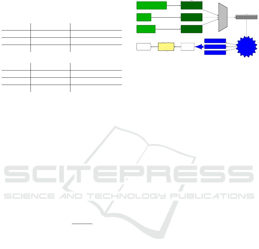
Table 3: Results of the clustering experiments for compari-

son. One can see an improvement over the baseline model

when using Autoencoder.

(a) HTTP clustering

Architecture Accuracy (dominant) Avg. Conﬁdence (dominant)

Baseline SOM 75% (75%) 58.34% (58.34%)

CNN + SOM 68.75% (68.75%) 53.61% (53.61%)

AE + SOM 87.5% (87.5%) 69.24% (69.24%)

(b) FTP clustering

Architecture Accuracy (dominant) Avg. Conﬁdence (dominant)

Baseline SOM 60.94% (72.22%) 51.8% (61.4%)

CNN + SOM 29.69% (29.69%) 18.19% (18.19%)

AE + SOM 67.19% (86%) 56.11% (71.82%)

ﬁrst multi-model approach. We compare three dif-

ferent conﬁgurations of self-organizing maps in terms

of their performance on our clustering metrics against

each other. Firstly, the 128 neuron-wide SOM will

use the encoding from the autoencoder model. Sec-

ondly, the 240 neuron-wide SOM will use the feature

maps of the CNN architecture. Lastly, as a baseline,

we use a raw SOM with 1024 neuron inputs for whole

statements.

We use two metrics to judge the effectiveness of

the clustering for each setup. The ﬁrst is accuracy:

how many detected clusters match a message type of

the protocol with more than 50% conﬁdence, which

will be referred to as a “dominant” cluster. Here, con-

ﬁdence is deﬁned as the relative share of a type among

all messages assigned to one cluster. If there are 120

messages of type A and 80 messages of type B, all

put into one cluster, then the conﬁdence of this clus-

ter to represent type A will be

120

120 + 80

= 60%. The

second metric is the average conﬁdence among all

clusters. Both metrics are also reported for dominant

types only (> 50% for one type), to remove empty

and small clusters from the average.

Table 3 shows the results of the experiments.

Some setups using dedicated feature extractors can

outperform the baseline signiﬁcantly. The autoen-

coder appears to be better suited for this task, perhaps

because the CNN architecture required a workaround

with data augmentation to even allow for training. For

further experiments that require cluster indexes, we

combine the AE and SOM architectures as a pipeline

to replace messages with their cluster index.

4.5 State Recognition

To recognize deeper states in a protocol, we use

the correlation of message sequences as they appear

chronologically in the dataset. For this, we replaced

HTTP/1.1 200 POST...

HTTP/1.1

200 OK...

HTTP/1.1 302

Moved...

HTTP/1.1

200 POST...

HTTP/1.1

200 OK...

HTTP/1.1

302 Moved...

1024 Chars/Bytes

Padding/Capping

Autoencoder

(AE)

HTTP/1.1...

128 Chars/Bytes

SOM

(16 Classes)

1 (POST)

4 (OK)

7 (Moved)

...

Sequence:

1, 7, 1

LSTM

Prediction:

Figure 7: This ﬁgure shows examples of HTTP statements

as they are processed for state recognition.

all messages with their cluster assigned by the cluster-

ing model. A simple LSTM with ﬁtting dimensions

to the SOM output is sufﬁcient to indicate highly cor-

related sequences by presenting the network’s conﬁ-

dence for what the following message type could be.

The central idea of SOM learning is arranging sim-

ilar types of messages in proximity to one another,

thereby allowing the use of the MSE loss function to

approximate the correct message type in the LSTM

output. The use of Cross-Entropy (CRE) loss has

shown no convergence. For training, we use an Adam

optimizer with a learning rate = 0.005 and betas =

(0.3, 0.9).

The setup is shown in ﬁgure 7. A simple time-

series prediction using a recurrent architecture shows

promising results in FTP, where actual states are im-

plied in the protocol. With the 64 indicated possi-

ble clusters, the LSTM matched 42% of the predicted

message types to the following actual message. This

number may seem low at ﬁrst glance; however, for an

in-depth state fuzzing approach using many attempts,

we view this as a signiﬁcant improvement over ran-

dom choice.

This experiment was also conducted for the HTTP

protocol, and the results are less impressive. Out of

the 16 implied clusters, 72% were correctly predicted.

This number may seem high at ﬁrst glance but relies

on predicting the average cluster number aligned with

the dataset bias. In other words, the prediction simply

states two or three alternating types for the GET mes-

sage, which drives the prediction accuracy higher than

any different prediction pattern. The dataset could

not be balanced for classes in this experiment, as we

wanted to avoid changing any sequential dependen-

cies by randomly picking messages. As a result, the

input data for HTTP has a signiﬁcant bias towards

GET message types, as the original data have, which

ultimately explains this behavior of the LSTM.

The results in this section showcase the potential

hazards of working with machine learning techniques,

mixing their embeddings and approaches, as well as

the interpretation of a predeﬁned metric. Even though

PREUNN: Protocol Reverse Engineering using Neural Networks

353

the results were a success in regard to the stateful pro-

tocol, which was our original aim for this experiment,

applying the same efforts to a stateless protocol shows

the weakness and dangerous pitfalls when interpret-

ing the metric. For both protocols, the metric is mis-

leading at face value. Only an analytic look at actual

prediction results did correct the error.

4.6 Sequence Generation

To fully mimic all aspects of the behavior of a pro-

tocol, we must be able to create syntactically cor-

rect messages with real-world distribution. We use

an LSTM model similar to the one for feature re-

verse engineering with added context. For any mes-

sage, instead of using a generic SOP and EOP symbol

as markers for beginning and end, we introduce new

special symbols, which are individualized by cluster

type. This results in 2 × 16 extra symbols for HTTP

and 2 × 64 additional symbols for FTP to be added to

the ASCII alphabet in their respective setups and sub-

sequently to the one-hot-encoding. The sequences put

into the LSTM, which uses a hidden size of 100 neu-

rons in two layers to account for the extra complexity,

have the beginnings and endings of each message in-

dicated by a cluster special SOP or EOP symbol. The

rest of the model architecture is identical to the one

used for feature reverse engineering, including con-

volutional embedding. Again, for training, we use the

Adam optimizer with a learning rate = 0.005 and de-

fault betas with an NLL loss function.

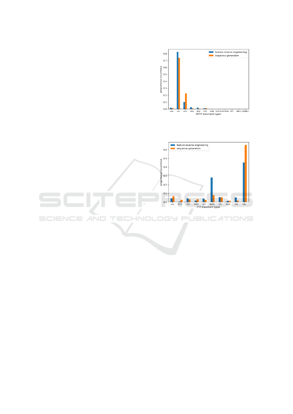
We use the same metric as for the feature re-

verse engineering LSTM. We parsed the generated

sequence into HTTP/FTP statements wrapped up in

some valid low-level protocol headers and collected

them in a pcap ﬁle. 63% of all sequences were iden-

tiﬁed as valid for HTTP and 100% for FTP by Wire-

shark. The excellent result on FTP is explainable for

the same reasons as in the feature reverse engineer-

ing, suffering from the simplicity of the messages and

training data. Figure 9 shows the type distribution of

both the feature reverse engineering and the sequence

generation for FTP to visualize the impact of adding

the other steps via cluster indexing. Only one class

stands out, which is either due to its simplicity or

a miscategorization of FTP types on our part. The

curve indicates, that a wider, more balanced distri-

bution of types was inferred. For the comparatively

lower HTTP result, as shown in ﬁgure 8, the messages

displayed a greater correlation between requests and

responses in the sequence generation. This implies

that the added context of types allows the neural net-

work to learn these connections more effectively. We

expect that more capable and larger architectures will

Figure 8: HTTP feature reverse engineering (blue) vs. se-

quence generation (orange) results in terms of type distri-

bution. Sequence generation shows better request/response

correlation.

Figure 9: FTP feature reverse engineering (blue) vs. se-

quence generation (orange) results in terms of type distribu-

tion. Sequence generation shows a better distribution except

for 1 class.

show an increase in the effectiveness of the observed

behavior.

This result lays the ﬁnal foundation we needed to

enable deep learning-based fuzzing of any protocol,

as a PRE approach is designed to be generally appli-

cable.

5 RELATED WORK

Learn&Fuzz: Machine Learning for Input

Fuzzing. Based on the idea that fuzzing only re-

quires an approximately correct input, the authors

of (Godefroid et al., 2017) used a recurrent neu-

ral network to help in fuzzing a PDF parser in a

browser. The syntax for objects, a central building

block of PDFs, was inferred by an AI in this work.

The authors used three different sampling strategies

from their network to address various challenges in

fuzzing: NoSample, Sample, and SampleSpace. The

ﬁrst one sees the RNN pick the letter with the highest

ICISSP 2022 - 8th International Conference on Information Systems Security and Privacy

354

score among the output to ensure syntactically cor-

rect objects. The second strategy takes the network’s

softmax output as a probability distribution for pick-

ing the next letter. This increases the fuzzing cover-

age but may result in many ill-formed objects. Lastly,

the SampleSpace strategy combines the two previous.

No-Sample is used until a whitespace is generated.

The next following character is sampled by proba-

bility, only to switch back to the No-Sample strat-

egy again. This creates more syntactically correct ob-

jects while also creating a more comprehensive mix

of different objects. These strategies were used in

the LSTM sampling. Our sampling, however, has to

cover message context as well.

Machine Learning for Black-box Fuzzing of Net-

work Protocols. The authors (Fan and Chang,

2017) see their work as the ﬁrst attempt to com-

bine an in-depth learning approach with black-box

fuzzing. They deploy a sequence-to-sequence model,

a two-part LSTM model invented for machine trans-

lation (Sutskever et al., 2014), to learn the seman-

tics of network protocols and create new output for

fuzzing purposes. Their work differs from this paper

in the number of steps taken and models employed to

learn details about the protocol. Here, a whole model

is presented, which was derived from previous work

on PRE. Additional information such as clustering or

context-based generation is missing as well.

GANFuzz: A GAN-based Industrial Network Pro-

tocol Fuzzing Framework. The GANFuzz Frame-

work (Hu et al., 2018) represents an alternative ap-

proach to protocol fuzzing using deep learning but

falls into the same category as the previous paper.

Instead of a sequence-to-sequence model, GANFuzz

uses a model known as a SequenceGAN (SeqGAN)

(Yu et al., 2017). This is a version of the common

GAN model but adjusted for text-based data using re-

inforcement learning. The authors of the paper train

one SeqGAN per message type, which they deduce

from a variety of clustering heuristics. This makes

their approach more similar to PREUNN but is still

missing several work steps, a concise work step mode,

and the generation of data done by context symbols

instead of entirely separate models.

Deep Neural Network-based Automatic Unknown

Protocol Classiﬁcation System Using Histogram

Feature. Jung and Jeong demonstrated a machine-

learning-based PRE approach to classify unknown

protocols (Jung and Jeong, 2020). They use statistical

methods to extract features from ten different proto-

cols and feed them into a deep belief network, clas-

sifying the message based on these features. Based

on the approach, they report a classiﬁcation accuracy

of about 99% on unknown datasets. Their method

differs from PREUNN in several ways. They semi-

automatically extract features using statistical meth-

ods, while we fully automated this process using an

autoencoder. Furthermore, their work’s goal is to

classify unknown protocol messages, whereas we aim

to generate new valid messages based on a novel pro-

tocol. Classiﬁcation in PREUNN happens implicitly.

Network Trafﬁc Classiﬁcation (NTC). The topic

of NTC is related to PRE regarding feature extraction.

Several papers are combining NTC with ML and NNs

(Lopez-Martin et al., 2017; Michael et al., 2017; Li

et al., 2018). However, the more complex steps of

PRE, like generating new packages for an unknown

protocol, are not addressed in those papers.

6 CONCLUSION

PREUNN represents a novel approach for the separa-

tion of traditional protocol reverse engineering tasks

that can be implemented using only neural networks.

In this paper, the widespread application layer proto-

col HTTP v1.1 and FTP were successfully reverse-

engineered using our approach. This highlights the

potential of several deep learning architectures such

as AEs for feature extraction, LSTMs for feature re-

verse engineering, SOMs for clustering, LSTMs for

state recognition, and ﬁnally a combination of the

above for sequence generation. The results achieved

include a decent, intuitively agreeable clustering and a

context-capable message generation model. We omit-

ted optimizations and testing the use of PREUNN for

fuzzing entirely due to time restraints and leave them

for future work. Our modular approach allows the use

of newer architectures from the ﬁelds of deep learn-

ing, such as natural language processing (e.g. BERT)

for improvements. Further future work could also in-

clude the use of reinforcement learning utilizing these

pre-trained models to create an automated fuzzer that

is capable of reverse engineering any similarly struc-

tured message-based language.

REFERENCES

Bac¸

ao, F., Lobo, V., and Painho, M. (2005). Self-organizing

maps as substitutes for k-means clustering. In Inter-

national Conference on Computational Science, pages

476–483. Springer.

Besic, N. (2019). What is a fuzzer and what does fuzzing

PREUNN: Protocol Reverse Engineering using Neural Networks

355

mean. https://www.neuralegion.com/fuzzing-what-

is-fuzzer/.

Brook, C. (2018). What is deep packet inspection?

how it works, use cases for dpi, and more.

https://digitalguardian.com/blog/what-deep-packet-

inspection-how-it-works-use-cases-dpi-and-more.

Caballero, J., Yin, H., Liang, Z., and Song, D. (2007). Poly-

glot: Automatic extraction of protocol message format

using dynamic binary analysis. In Proceedings of the

14th ACM conference on Computer and communica-

tions security, pages 317–329.

Comparetti, P. M., Wondracek, G., Kruegel, C., and Kirda,

E. (2009). Prospex: Protocol speciﬁcation extraction.

In 2009 30th IEEE Symposium on Security and Pri-

vacy, pages 110–125. IEEE.

Cui, W., Kannan, J., and Wang, H. J. (2007). Discoverer:

Automatic protocol reverse engineering from network

traces. In USENIX Security Symposium, pages 1–14.

Duchene, J., Le Guernic, C., Alata, E., Nicomette, V., and

aniche, M. (2018). State of the art of network pro-

tocol reverse engineering tools. Journal of Computer

Virology and Hacking Techniques, 14(1):53–68.

Fan, R. and Chang, Y. (2017). Machine learning for black-

box fuzzing of network protocols. In International

Conference on Information and Communications Se-

curity, pages 621–632. Springer.

Garﬁnkel, S. (2008). Nitroba university harassment sce-

nario. Dataset: https://digitalcorpora.org/corpora/

scenarios/nitroba-university-harassment-scenario.

Godefroid, P., Peleg, H., and Singh, R. (2017). Learn&fuzz:

Machine learning for input fuzzing. In 2017 32nd

IEEE/ACM International Conference on Automated

Software Engineering (ASE), pages 50–59. IEEE.

Goo, Y.-H., Shim, K.-S., Lee, M.-S., and Kim, M.-S.

(2019). Http and dns trafﬁc traces for experiment-

ing of protocol reverse engineering methods. http:

//dx.doi.org/10.21227/tpqf-fe98.

Goodfellow, I., Pouget-Abadie, J., Mirza, M., Xu, B.,

Warde-Farley, D., Ozair, S., Courville, A., and Ben-

gio, Y. (2014). Generative adversarial nets. In

Advances in neural information processing systems,

pages 2672–2680.

Hinton, G. E. and Salakhutdinov, R. (2006). Reducing the

dimensionality of data with neural networks. Science,

313:504 – 507.

Hochreiter, S. and Schmidhuber, J. (1997). Long short-term

memory. Neural computation, 9(8):1735–1780.

Hornik, K., Stinchcombe, M., White, H., et al. (1989). Mul-

tilayer feedforward networks are universal approxi-

mators. Neural networks, 2(5):359–366.

Hu, Z., Shi, J., Huang, Y., Xiong, J., and Bu, X. (2018).

Ganfuzz: a gan-based industrial network protocol

fuzzing framework. In Proceedings of the 15th ACM

International Conference on Computing Frontiers,

pages 138–145.

Jung, Y. and Jeong, C.-M. (2020). Deep neural network-

based automatic unknown protocol classiﬁcation sys-

tem using histogram feature. The Journal of Super-

computing, 76(7):5425–5441.

Kohonen, T. (1982). Self-organized formation of topolog-

ically correct feature maps. Biological cybernetics,

43(1):59–69.

Krizhevsky, A., Sutskever, I., and Hinton, G. E. (2012).

Imagenet classiﬁcation with deep convolutional neu-

ral networks. In Pereira, F., Burges, C. J. C., Bottou,

L., and Weinberger, K. Q., editors, Advances in Neu-

ral Information Processing Systems 25, pages 1097–

1105. Curran Associates, Inc.

Lang, K. J. (1999). Faster algorithms for ﬁnding minimal

consistent dfas. NEC Research Institute, Tech. Rep.

Li, R., Xiao, X., Ni, S., Zheng, H., and Xia, S. (2018). Byte

segment neural network for network trafﬁc classiﬁca-

tion. In 2018 IEEE/ACM 26th International Sympo-

sium on Quality of Service (IWQoS), pages 1–10.

Lopez-Martin, M., Carro, B., Sanchez-Esguevillas, A., and

Lloret, J. (2017). Network trafﬁc classiﬁer with con-

volutional and recurrent neural networks for internet

of things. IEEE Access, 5:18042–18050.

Michael, A., Valla, E., Neggatu, N. S., and Moore, A.

(2017). Network trafﬁc classiﬁcation via neural net-

works. Technical Report UCAM-CL-TR-912, Univer-

sity of Cambridge, Computer Laboratory.

Narayan, J., Shukla, S. K., and Clancy, T. C. (2015). A sur-

vey of automatic protocol reverse engineering tools.

ACM Computing Surveys (CSUR), 48(3):1–26.

Pang, R. and Paxson, V. (2003). Lawrence Berkeley Na-

tional Laboratory - FTP - Packet Trace. Dataset:

https://ee.lbl.gov/anonymized-traces.html.

Radford, A., Metz, L., and Chintala, S. (2015). Unsu-

pervised representation learning with deep convolu-

tional generative adversarial networks. arXiv preprint

arXiv:1511.06434.

Selvaraju, R. R., Cogswell, M., Das, A., Vedantam, R.,

Parikh, D., and Batra, D. (2017). Grad-cam: Visual

explanations from deep networks via gradient-based

localization. In Proceedings of the IEEE international

conference on computer vision, pages 618–626.

Sharafaldin, I., Lashkari, A. H., Hakak, S., and Ghorbani,

A. A. (2019). Developing realistic distributed denial

of service (ddos) attack dataset and taxonomy. In 2019

International Carnahan Conference on Security Tech-

nology (ICCST), pages 1–8. IEEE.

Shiravi, A., Shiravi, H., Tavallaee, M., and Ghorbani, A. A.

(2012). Toward developing a systematic approach to

generate benchmark datasets for intrusion detection.

computers & security, 31(3):357–374.

Sutskever, I., Vinyals, O., and Le, Q. V. (2014). Se-

quence to sequence learning with neural networks. In

Advances in neural information processing systems,

pages 3104–3112.

TC97, I. (1984). Basic reference model. International Stan-

dard, ISO/IS, 7498.

Wondracek, G., Comparetti, P. M., Kruegel, C., and Kirda,

E. (2008). Automatic network protocol analysis. In

NDSS, volume 8, pages 1–14.

Yu, L., Zhang, W., Wang, J., and Yu, Y. (2017). Seqgan:

Sequence generative adversarial nets with policy gra-

dient. In Thirty-ﬁrst AAAI conference on artiﬁcial in-

telligence.

ICISSP 2022 - 8th International Conference on Information Systems Security and Privacy

356