Formal Scenario-driven Logical Spaces for Randomized Synthetic Data

Generation

Osama Maqbool and J

urgen Roßmann

Institute for Man-Machine-Interaction, RWTH Aachen University, Germany

Keywords:

Logical Scenarios, Randomization, Synthetic Data.

Abstract:

Simulations and synthetic data are a necessary supplement to real-world experiments in order to alleviate its

effort, cost and risks. As demand of data for development and validation increases, simulations too must cor-

respondingly be scaled. Variation of simulation parameters affords simulation designers control over the scope

of how a simulation is scaled— they can chose a balance between target distribution of simulation variants

and the degree of randomness— thereby achieving both the volume and diversity of synthetic data. This paper

proposes logical scenarios as basis for simulation variation. Scenarios are formal human-readable scripts of

simulations and test drives used within the automotive industry. They are deﬁned at different abstraction lev-

els, one of which is the logical scenario as a parameterized simulation model with description for parameters

instead of concrete values. This contribution proposes methodologies to model the parameter descriptions in a

modular fashion with parameter ranges, probability distributions and inter-relations. A randomization engine

is introduced based on Markov chain Monte-Carlo methods to efﬁciently sample the modeled space. The re-

sult is a variety of simulation-independent concrete scenarios that follow the formal scenario speciﬁcation.

1 INTRODUCTION

The growth of intelligent systems in various opera-

tional domains is marked by a signiﬁcant increase

in the complexity of systems, which has created de-

mands for new and innovative strategies throughout

the system life-cycle: from development through vali-

dation to maintenance. Based often on Artiﬁcial Intel-

ligence, complex systems depend on diverse and am-

ple training data, and the high complexity also neces-

sitates a validation strategy in a large number of op-

erational situations. Case in point is the Automobile

Industry, where Wachenfeld and Winner (Wachenfeld

and Winner, 2016) estimate 6.62 billion test kilome-

ters for the validation of autonomous driving func-

tions.

A natural alternative to costly real-world experi-

ments is generating synthetic data from simulations.

This is achieved in a number of examples in dif-

ferent ways. A single or set of parameters may be

varied per a given distribution to study a particular

aspect of the whole system (Wagner et al., 2018),

the operational domain of a system may be random-

ized (Khirodkar et al., 2019), or a systematic varia-

tion approach may be built up allowing the designer

full control over data distribution (Ben Abdessalem

et al., 2016). This contribution considers a formal

scenario-based approach (Menzel et al., 2018) cou-

pled with digital twins for generating synthetic data

in a systematic manner. Scenarios are used within

the automotive industry as standardized descriptions

of a scene ﬂow and are used mainly for validation

of complex Automated Driving Systems (ADS). Sce-

narios can be parameterized to create logical spaces,

wherein parameter values may be varied to gener-

ate a variety of concrete scenarios. This method of

parameter variation offers various advantages: a) it

works with simulation-independent and standardized

formats for describing situations, b) it generates se-

mantically correct data i.e. a valid scenario, and c)

it has potential applicability throughout the develop-

ment life-cycle due to the inherent integrate-ability of

scenarios throughout the cycle (Sippl et al., 2019).

This paper proposes a layered approach for mod-

eling the logical space of scenarios — speciﬁed via

a test speciﬁcation — a proposed addition to for-

mal scenario speciﬁcations. Parameters may be mod-

eled using reusable building blocks in a piece-wise

manner, with corresponding probability distributions,

and may be constrained together via inter-parameter

constraints. A randomization engine is introduced

to sample the multi-dimensional parameter space (or

Maqbool, O. and Roßmann, J.

Formal Scenario-driven Logical Spaces for Randomized Synthetic Data Generation.

DOI: 10.5220/0010816400003119

In Proceedings of the 10th International Conference on Model-Driven Engineering and Software Development (MODELSWARD 2022), pages 203-210

ISBN: 978-989-758-550-0; ISSN: 2184-4348

203

logical space) via variants of Markov chain Monte-

Carlo Sampling. The resulting concrete scenarios are

brought to life in a multi-domain 3D simulation en-

gine, within which the complete framework is inte-

grated as a dynamic library.

The rest of the paper is organized as follows. Sec-

tion 2 presents the related work, Section 3 gives an

overview of different types of scenarios. Section 4

explains in detail the modeling approach for logical

spaces and corresponding sampling methods. Section

5 presents two exemplary cases from the automotive

domain, and Section 6 concludes the work.

2 RELATED WORK

Variation or randomization of simulation parameters

has different purposes. One of the most common ap-

plications is the sensitivity analysis (Hartjen et al.,

2019) of parameters. Within machine learning appli-

cations, domain randomization (Tobin et al., 2017) is

used to increase the diversity of data and is especially

beneﬁcial in transfer learning applications. Genera-

tive Adversarial Neural Networks are neural networks

(Goodfellow et al., 2014) that may be trained to gen-

erate synthetic data targeted towards challenging the

system under training.

Systematic variation approaches target solely on

the variation aspect and attempt to build models or

grammar which inherently cater to the semantic cor-

rectness of a scenario. (Jiang et al., 2018) devel-

oped a stochastic grammar, which combined with

a photo-realistic simulator yields valid 2D and 3D

scenes. (Bagschik et al., 2018) developed an ontology

for knowledge representation of automotive scenarios

from which varied trafﬁc scenes can be derived. (Feng

et al., 2021) identiﬁes decision parameters from a sce-

nario description, and uses criticality metrics based on

the decision variables to generate a testing scenario li-

brary.

Domain Speciﬁc Languages (DSL) provide users

with a programming framework where the scenario

execution can be described with value and probabil-

ity distribution constraints. ASAM OpenScenario 2.0

standard (ASAM, 2021c) follows this approach. A

comparable approach is the Scenic language (Fre-

mont et al., 2019), a probabilistic programming lan-

guage (PPL) designed for automotive scenarios. PPLs

allow construction of probability distributions via ex-

pressive conditional constraints between variables.

(Fremont et al., 2020) uses the formal probabilistic

description in Scenic for test-case generation of au-

tonomous vehicle safety scenarios.

DSLs with PPL-like attributes provide both ex-

pressiveness and a detailed control over design of

variation space. However, the mentioned approaches

are lacking on mathematical constraints between vari-

ables, which are crucial for 3D simulation, e.g. to

place bounds on variation of trajectories and object

geometries. This contribution focuses on the mathe-

matical relations and inference techniques to samples

with such constraints.

3 BACKGROUND ON

SCENARIOS

Formal scenarios considered within this contribution

were introduced in the PEGASUS project (Winner

et al., 2019) as a validation strategy for complex au-

tomotive systems. A scenario is a simulation script

or story, formally deﬁned as “the temporal develop-

ment between several scenes in sequence of scenes”,

enriched by entities, actions and events, goals and val-

ues (Ulbrich et al., 2015).

3.1 Abstraction Levels

(Menzel et al., 2018) proposes three levels of scenario

abstraction: functional, logical and concrete scenar-

ios. Functional scenarios are at the highest level

of abstraction, composed of semantic information in

natural language, providing a common platform for

cross-domain experts. On the other end, a concrete

scenario contains state space variables and concrete

parameters describing the environment, entities and

their relations to each other. Logical scenarios are in

the middle; they contain the state space variables de-

scribing the environment, entities and relations, but

describe parameter ranges instead of concrete values.

3.2 Randomizing Scenarios

The logical space offers a systematic playground to

specify variations of a scenario. Figure 1 illustrates

a modeling approach for an automotive scenario.

The static and dynamic aspects are typically speci-

ﬁed via the ASAM OpenDRIVE (ASAM, 2021a) and

OpenSCENARIO (ASAM, 2021b) standards respec-

tively. The test speciﬁcation ﬁle is a proposed addi-

tion to the formal scenario speciﬁcation, an XML-ﬁle

which refers to parameters within existing speciﬁca-

tion ﬁles, along with their ranges, probability distri-

butions, parameter- and inter-parameter constraints,

thereby providing a systematic modeling approach for

the logical space. Once modeled, a randomization en-

gine is proposed as the variation methodology to gen-

erate concrete scenario variants based on the logical

MODELSWARD 2022 - 10th International Conference on Model-Driven Engineering and Software Development

204

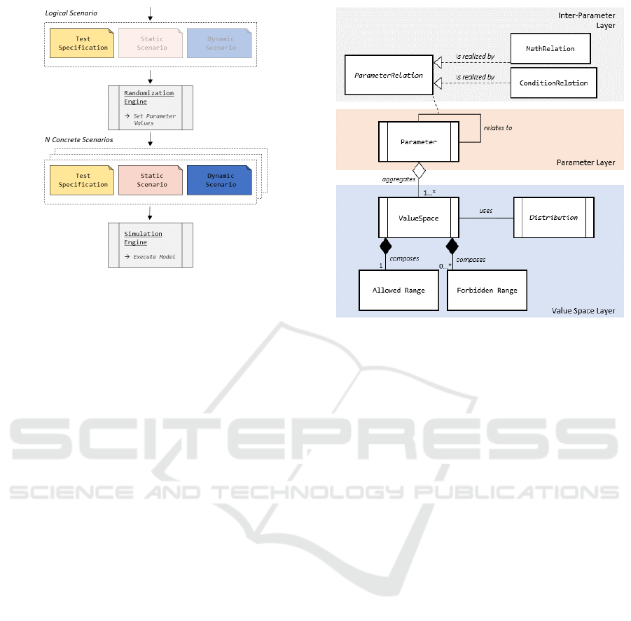
Figure 1: Test speciﬁcation based description of logical sce-

narios.

space speciﬁcation. The randomization engine uses

Monte-Carlo based sampling of the modeled logical

space. It works independently of the scenarios them-

selves, and is capable of taking mathematical and con-

ditional constraints into account to sample from the

speciﬁed distributions.

4 MODELING AND SAMPLING

LOGICAL SPACES

A concrete scenario consists of a sequence of input

data ¯u(t), e.g. sensor data, initial states ¯s

and param-

eters ¯p. Based on the data, a simulation engine uses a

digital twin M of a system to generate state trajecto-

ries.

¯s(t) = M( ¯s

, ¯u(t), ¯p, t) ¯s, ¯s

∈ S, ¯u ∈ U, ¯p ∈ L (1)

S, U, L are the domains of their respective vari-

ables. In order to create variants of concrete scenar-

ios, one can thus vary the static elements ¯p by tak-

ing samples from L.The initial state values ¯s

are also

static and can be varied in a similar fashion. There-

from follows the formal deﬁnition for logical space

modeling:

Logical space modeling is the modeling of

L, i.e. constituent values, constraining con-

ditions and probability distribution functions

that dictate whether and how often a value

may be drawn.

Figure 2: Layered approach for logical space modeling. Re-

lations are read from left to right or top to bottom.

4.1 Modeling Methodology

The approach for modeling logical space L is illus-

trated in Figure 2. Starting from bottom to top, each

layer builds some part of the logical space, and subse-

quent layers use the pre-built spaces to construct more

complex spaces. Each layer is self-contained, and

can be used independently to generate samples. The

ﬁgure serves as a modeling guideline as well as the

software architecture for the test speciﬁcation reader,

which must parse the XML elements and create corre-

sponding entities (e.g. C++ objects). These are subse-

quently used by the randomization engine to generate

samples (see Section 4.2).

4.1.1 Value Space Layer

This layer is the basic building block of the logical

space. A value space is a continuous range or a dis-

crete set from which a single parameter may draw val-

ues. The space is deﬁned by allowed and forbidden

ranges (or sets for discrete parameters). A probabil-

ity distribution must be speciﬁed at this level to dic-

tate how samples shall be drawn from the value space.

Figure 3 illustrates a value space speciﬁed in the test

speciﬁcation for the speed of a vehicle on a highway,

deﬁned with an allowed and forbidden range, and a

gaussian probability distribution.

Formal Scenario-driven Logical Spaces for Randomized Synthetic Data Generation

205

Figure 3: Value space in the test speciﬁcation.

4.1.2 Probability Distribution

The probability distribution can be speciﬁed individu-

ally for each parameter, or a multi-variate distribution

may be speciﬁed for multiple parameters. The distri-

bution can be derived from user knowledge as analyt-

ical models or from data as data-driven functions, and

it must be implemented within the test speciﬁcation

reader inheriting from Distribution (see Figure 2). It

can then be referred to in the test speciﬁcation XML.

Example is the gaussian distribution speciﬁed in Fig-

ure 3.

4.1.3 Parameter Layer

Whereas value spaces have no direct meaning for the

system per se, parameters refer to the properties of a

concrete digital twin a system (and thereby also the

real system). The same value space may be used by

multiple parameters and multiple value spaces may be

used by the same parameter, each with its occurrence

likelihood. The multiplicity of value spaces allow the

creation of discontinuous parameter ranges, diversi-

ﬁed probability distributions and isolation of different

operational domains of a parameter. Figure 4 illus-

trates an example of the parameter vehicle speed of a

given ego vehicle, which may sample from two value

spaces with an equal likelihood.

Figure 4: Parameter speciﬁcation in the test speciﬁcation.

4.1.4 Inter-Parameter Layer

The Inter-Parameter Layer allows the binding of

various parameters through inter-parameter relations.

Two types of relations are possible.

Mathematical Constraints: The parameters p

can

be bounded with each other via mathematical con-

straints

( ¯p) =

(

g( ¯p) = 0

e( ¯p) ≥ 0,

(2)

where g and h specify the mathematical equalities

and inequalities respectively. An example of mathe-

matical constraints is illustrated in Figure 5 within the

XML-Tag MathRelation: speed of vehicle 1 must be

greater than that of vehicle 2 by at least 5 km/h during

an overtake scenario:

Figure 5: Speciﬁcation of inter-parameter constraints.

Conditional Constraints: Conditional here refers

to the technical term in computer science, realized e.g.

as If-Then-Else type constructs in programming lan-

guages.

( ¯p) :

IF (p

= a ∧ p

∈ [b, c])

THEN (p

∈ [x, y])

(3)

The conditional constraints must be formulated

such that for a given set of concrete parameter val-

ues, all constraints C

can be evaluated to either true

or false. The XML-Tag CondRelation in Figure 5 il-

lustrates an example of a conditional relation: regard-

less of the speciﬁed distributions of vehicle speeds in

a scenario, they must be zero if the parameter “state

of trafﬁc signal” is equal to “RED”.

4.2 Generating Samples

Generating samples from L is achieved via a random-

ization engine, a task equivalent to making inferences

about probability distributions. Harmonic with the

layered modeling approach, samples can be drawn

for each parameter individually or from the complete

multi-dimensional constrained space.

4.2.1 Sampling Value Spaces

Rejection sampling is used for drawing samples from

value spaces. Samples are drawn from the speciﬁed

distribution, and accepted only if the fall within the

speciﬁed ranges.

MODELSWARD 2022 - 10th International Conference on Model-Driven Engineering and Software Development

206

4.2.2 Sampling Parameters

Based on the occurrence frequency, an underlying

value space is chosen, and its local sampling function

is used to generate a sample.

4.2.3 Sampling Constrained Logical Space

The constrained logical space L consists of all the pa-

rameters as well as their inter-relations. The sampling

problem can be formulated in terms of a target distri-

bution f

over the parameter vector ¯p:

( ¯p) =

(

( ¯p) C

( ¯p) = 1 ∧ C

( ¯p) = 1

0 otherwise,

(4)

( ¯p) and C

( ¯p) are the mathematical and con-

ditional relations respectively. f

is the distribution

speciﬁed by the user, e.g. the gaussian distribution

speciﬁed in Figure 3. The target distribution differs

from the speciﬁed distribution in that it also takes

parameter constraints into account. It is equal to f

when constraints hold and drops to zero otherwise.

Samples therefore have to be drawn from the target

distribution f

, it is however not directly sample-able.

Rejection sampling, i.e. directly sampling from

and rejecting samples violating constraints, is an

obvious but inefﬁcient candidate as the constraints

may exclude high frequency areas of the speciﬁed

distribution, leading to a very high rejection rate.

To efﬁciently handle such conﬂicts, two variants of

the Markov Chain Monte-Carlo (MCMC) method are

used which draw from a distribution that approxi-

mates f

. Essentially, they prescribe random sam-

pling (the Monte-Carlo part) using a proposal distri-

bution. The samples are drawn sequentially such that

the acceptance of any sample is dependent on its prob-

ability with respect to the target distribution, relative

to the previous sample, thus forming a Markov Chain.

4.2.4 Resolving Mathematical Constraints with

Metropolis Algorithm

The Metropolis algorithm (Roberts, 1996) is used by

randomization engine to resolve linear mathematical

constraints C

and approximate the target distribu-

tion f

. The approach is based on (Van den Meersche

et al., 2009), and has the following steps:

1. Choose a Mathematical Sub-space: A single

value space from each parameter is chosen for

every iteration. The linear inter-parameter con-

straints, as well as the allowed and forbidden

ranges of each value space are expressed as ma-

trices G and E.

(a) Metropolis algorithm with

different linear constraints.

(b) Gibbs algorithm with

different non-linear con-

straints.

( ¯p) =

(

G ¯p = h

E ¯p ≥ f.

(5)

This step is the prepping of the problem for

Metropolis algorithm.

2. Draw Random Points: A set of random points

is generated such that they satisﬁes C

by sam-

pling from a proposal distribution. This random

sampling is done via xsample(), an R function for

solving linear inverse problems (Van den Meer-

sche et al., 2009). The algorithm ﬁrstly eliminates

the equality constraints G ¯p = h by transforming

the parameter vector ¯p into a vector ¯p

∗

with lin-

early independent elements.

¯p = ¯p

+ Q ¯p

∗

(6)

Where ¯p

is a solution of G ¯p = h and Q serves as

a basis for the null space of G, such that Q

⊤

Q =

I and GQ = 0. Thus the boundaries are reduced

to a set of inequalities

EQ ¯p

∗

≥ f − E ¯p

. (7)

These inequalities are in-fact hyper-planes bound-

ing the area of interest. Given an initial point that

is within the hyper-planes, subsequent points are

sampled sequentially, each dependent on last and

each random. To generate a random point z

from

a given point z

, candidate z

∗

is chosen by an ar-

bitrary line from z

with length sampled from a

normal distribution.

∗

= z

+ η (8)

Formal Scenario-driven Logical Spaces for Randomized Synthetic Data Generation

207

If z

∗

lies within the inequalities in Equation 7,

it is accepted as a valid sample z

. Otherwise,

the point is “mirrored” across the ﬁrst hyper-plane

that intersects this line. If the new point lies within

the bounds, it is accepted, otherwise the process is

repeated.

The random walk using the mirror algorithm en-

sures that the points are generated from a symmet-

ric distribution as required by MCMC, along with

a high acceptance rate.

3. Map Random Points to Target Distribution:

With a set of random points that all satisfy C

, a

subset of the points is mapped to f

. This is done

sequentially with the MCMC criterion. Given a

point z

and a previously accepted point z

, if

)

>= r, (9)

then the point is accepted, otherwise rejected, r

being between 0 and 1. The process is then re-

peated.

Samples within an initial burn-in phase are typically

ignored until the Markov chain converges to the tar-

get distribution. The choice of r is also important to

set the exploration-exploitation balance of the algo-

rithm — whether it converges quickly to a local peak

or chooses to explore low-density areas as well.

The algorithm results are illustrated in Figure 6a.

Red lines denote the bounding constraints. Working

with relative frequencies allow the algorithm to re-

duce rejection ratio yet still converge as best as possi-

ble to the speciﬁed distribution.

Non-linear Constraints: For non-linear, espe-

cially non-convex bounds, step 2 becomes a chal-

lenge. For this, another algorithm is introduced in the

next section which bypasses this step altogether.

4.2.5 Resolving Conditional Constraints with

Metropolis within Gibbs Algorithm

The Gibbs algorithm (Smith and Roberts, 1993) is

also a variant of the MCMC methods targeted more

towards multivariate distributions. The algorithm

uses the conditional probabilities rather than the joint

probability and is capable of handling non-linear con-

straints, conditional constraints and both at the same

time. The randomization engine applies a more robust

variant, the “Metropolis within Gibbs” algorithm , in

the following steps:

1. For the target distribution in Equation 4, choose a

valid initial sample for ¯p. This is done via rejec-

tion sampling.

¯p

= (p

, p

, ..., p

) (10)

2. Draw a sample for the ﬁrst variable based on the

previous values of other variable samples:

, ..., p

). (11)

Since f

cannot be sampled directly, the sample

is drawn with the Metropolis algorithm, albeit dif-

ferently than before:

(a) Choose a random value for p

without taking

into account inter-parameter constraints C

and

(b) For a concrete sample p

∗

, accept the sample if

∗

, ..., p

)

, ..., p

)

> r, (12)

otherwise reject it. This is the step where the

constraints are taken into account. Since con-

straints C

are mathematical equalities and in-

equalities, and constraints C

are conditional

statements, evaluation of both must return ei-

ther true ( f

is equal to f

) or false ( f

is zero).

3. Draw a sample for the rest of the variables sim-

ilarly, using the new value of the previous vari-

ables in the conditional distribution in Equation

12. This completes one iteration, i.e. one com-

plete sample. The complete process is then re-

peated for further samples.

Figure 6b illustrates the results of Metropolis

within Gibbs, where the sampler converges to a nor-

mal distribution while being bounded within a 2-D

torus.

The Metropolis within Gibbs method offers more

ﬂexibility than the Metropolis method, as a random

sample is drawn ﬁrst and then checked for constraints,

making constraint handling simpler. Unlike Metropo-

lis, this order is feasible here as variation takes place

one dimension at a time, decreasing the likelihood of

invalid samples. However, the algorithm is compu-

tationally expensive, and puts additional requirement

on the implementation of Distribution, namely the

calculation of conditional distributions.

5 EXAMPLES

As examples, scenario-based logical space sampling

is applied to two automotive use-cases. The resulting

concrete scenarios contain the initial states and pa-

rameters for digital twins which are simulated within

the 3D simulation framework VEROSIM (Rossmann

et al., 2013). The simulation framework is equipped

to generate ground-truth sensor- and trajectory data

that can be used to bridge the data requirements for

training and validation purposes.

MODELSWARD 2022 - 10th International Conference on Model-Driven Engineering and Software Development

208

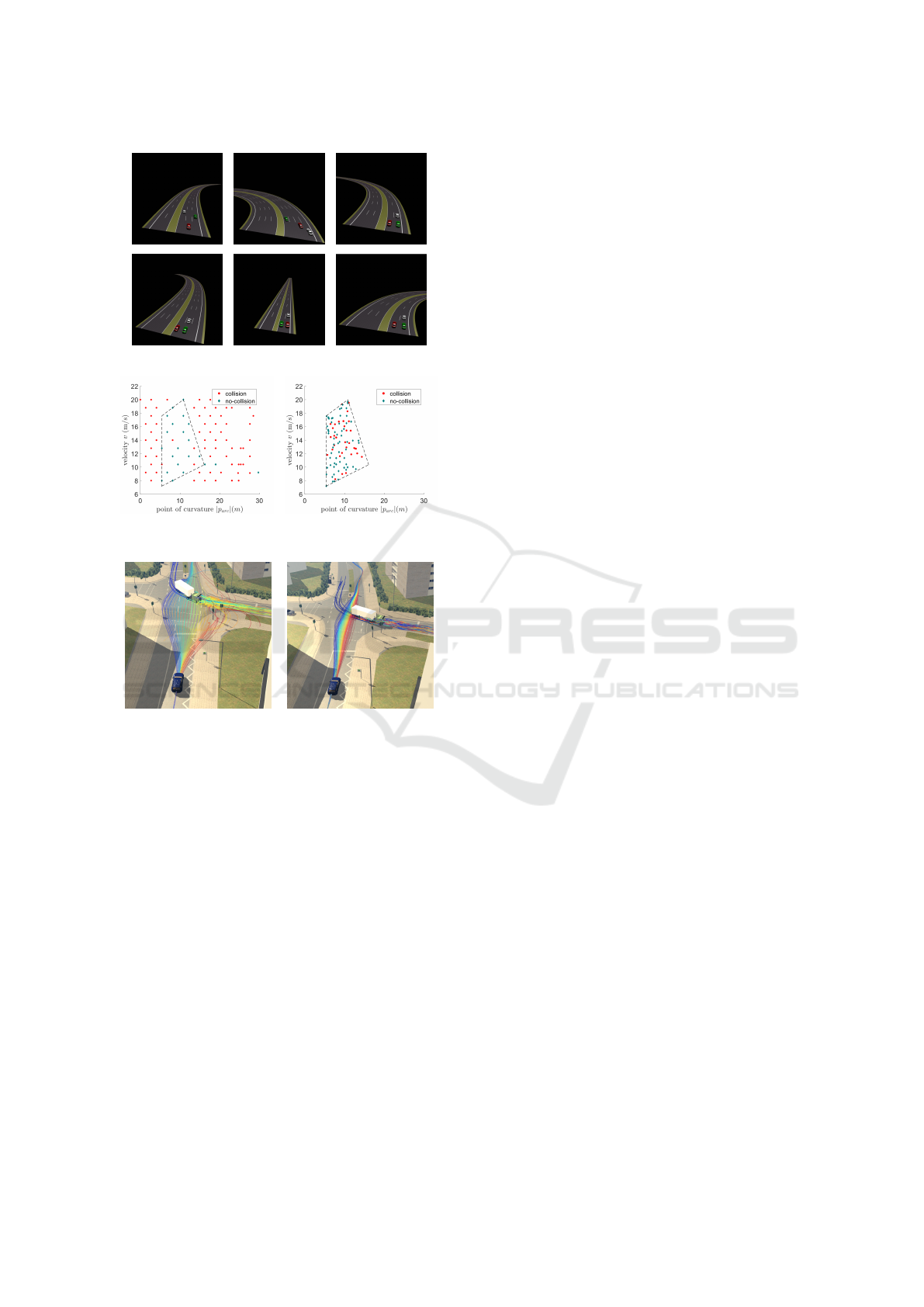
Figure 7: Randomizing static aspects of a scenario.

(a) Complete parameter

space exploration.

(b) Targeted parameter

space exploration.

plete parameter space.

(d) Simulation of the tar-

geted parameter space.

Figure 8: Investigating safe evasive maneuvers by random-

izing the dynamic scenario.

5.0.1 Randomizing Static Scenarios

Figure 7 illustrates an example of road layout ran-

domization, speciﬁed by the OpenDRIVE and Open-

SCENARIO formats. In this simple example, discrete

value sets with random distributions are assigned to

each of the following parameters of the scenario de-

scription: the road curvature, number of lanes, width

of lanes and the initial coordinates of trafﬁc partici-

pants. No inter-parameter relations are speciﬁed. The

resulting variety of concrete scenarios can then serve

as basis for simulation within different environments.

5.0.2 Randomizing Dynamic Scenarios

Randomization of a dynamic scenario is illustrated in

Figure 8 (based on a scenario from (Atorf and Roß-

mann, 2018)). An autonomous car approaches a road

intersection while an oncoming truck takes a turn, cut-

ting the path of the car. Given a constant behavior of

the truck, the car must perform an evasive maneuver

to avoid a collision.

The car drives with a velocity v based on a set of

target path points, out which the point of curvature

arc

can be varied to achieve an evasive maneuver.

The logical space modeling is done in two steps:

1. Firstly, the logical space is speciﬁed for the pa-

rameters v and p

arc

by specifying feasible ranges

and assigning a uniform distribution to each pa-

rameter. The simulations of the resulting concrete

scenarios gives an overview of the collision and

no-collision parameter regions, illustrated in Fig-

ure 8a. Figure 8c shows the simulated vehicle tra-

jectories.

2. With an overview of the overall parameter space

characteristics, regions more likely to result in the

desired outcome (lower collisions) are isolated.

This is done by adding mathematical constraints

between v and p

arc

. These constraints are illus-

trated in Figure 8b as lines bounding the region

of interest. The results are a higher ratio of no-

collision points as well as the cleaner trajectory

paths in the simulation in Figure 8d. Thus a de-

tailed insight into the effects of parameter varia-

tion are achieved via iterative logical space mod-

eling.

6 CONCLUSIONS

This contribution introduced a systematic framework

for modeling logical scenarios and using them as a

basis for parameter variation and simulation indepen-

dent generation of diverse synthetic data. The XML-

based test speciﬁcation of logical scenarios allows a

direct integration with formal scenario-based simu-

lations, but is not restricted to these. A promising

area of further research is the incorporation of the

proposed framework within existing domain speciﬁc-

and probabilistic programming languages in order to

provide the designer not just low level constraints in-

troduced here, but also higher-level modeling rules for

description of the complete scenario.

ACKNOWLEDGEMENTS

This work is part of the project “KImaDiZ”, sup-

ported by the German Aerospace Center (DLR) with

funds of the German Federal Ministry of Economics

and Technology (BMWi), support code 50 RA 1934.

Formal Scenario-driven Logical Spaces for Randomized Synthetic Data Generation

209

REFERENCES

ASAM (2021a). Asam opendrive. https://www.asam.net/

standards/detail/opendrive/. Accessed: 2021-08-10.

ASAM (2021b). Asam openscenario. https://www.asam.

net/standards/detail/openscenario/. Accessed: 2021-

08-10.

ASAM (2021c). Asam openscenario 2.0. https://www.

asam.net/project-detail/asam-openscenario-v20-1/.

Accessed: 2021-09-08.

Atorf, L. and Roßmann, J. (2018). Interactive analysis and

visualization of digital twins in high-dimensional state

spaces. In 2018 15th International Conference on

Control, Automation, Robotics and Vision (ICARCV),

pages 241–246. IEEE.

Bagschik, G., Menzel, T., and Maurer, M. (2018). Ontol-

ogy based scene creation for the development of au-

tomated vehicles. In 2018 IEEE Intelligent Vehicles

Symposium (IV), pages 1813–1820.

Ben Abdessalem, R., Nejati, S., Briand, L. C., and Stifter,

T. (2016). Testing advanced driver assistance systems

using multi-objective search and neural networks. In

2016 31st IEEE/ACM International Conference on

Automated Software Engineering (ASE), pages 63–74.

Feng, S., Feng, Y., Yu, C., Zhang, Y., and Liu, H. X.

(2021). Testing scenario library generation for con-

nected and automated vehicles, part i: Methodology.

IEEE Transactions on Intelligent Transportation Sys-

tems, 22(3):1573–1582.

Fremont, D. J., Dreossi, T., Ghosh, S., Yue, X.,

Sangiovanni-Vincentelli, A. L., and Seshia, S. A.

(2019). Scenic: A language for scenario speciﬁca-

tion and scene generation. In Proceedings of the 40th

ACM SIGPLAN Conference on Programming Lan-

guage Design and Implementation, PLDI 2019, page

63–78, New York, NY, USA. Association for Comput-

ing Machinery.

Fremont, D. J., Kim, E., Pant, Y. V., Seshia, S. A., Acharya,

A., Bruso, X., Wells, P., Lemke, S., Lu, Q., and

Mehta, S. (2020). Formal scenario-based testing of

autonomous vehicles: From simulation to the real

world. In 2020 IEEE 23rd International Conference

on Intelligent Transportation Systems (ITSC), pages

1–8.

Goodfellow, I., Pouget-Abadie, J., Mirza, M., Xu, B.,

Warde-Farley, D., Ozair, S., Courville, A., and Ben-

gio, Y. (2014). Generative adversarial nets. Advances

in neural information processing systems, 27.

Hartjen, L., Philipp, R., Schuldt, F., Friedrich, B., and

Howar, F. (2019). Classiﬁcation of driving maneuvers

in urban trafﬁc for parametrization of test scenarios.

In 9. Tagung Automatisiertes Fahren.

Jiang, C., Qi, S., Zhu, Y., Huang, S., Lin, J., Yu, L.-F., Ter-

zopoulos, D., and Zhu, S.-C. (2018). Conﬁgurable 3d

scene synthesis and 2d image rendering with per-pixel

ground truth using stochastic grammars. International

Journal of Computer Vision, 126(9):920–941.

Khirodkar, R., Yoo, D., and Kitani, K. (2019). Domain ran-

domization for scene-speciﬁc car detection and pose

estimation. In 2019 IEEE Winter Conference on Ap-

plications of Computer Vision (WACV), pages 1932–

1940.

Menzel, T., Bagschik, G., and Maurer, M. (2018). Scenarios

for development, test and validation of automated ve-

hicles. In 2018 IEEE Intelligent Vehicles Symposium

(IV), pages 1821–1827. IEEE.

Roberts, G. O. (1996). Markov chain concepts related to

sampling algorithms. Markov chain Monte Carlo in

practice, 57:45–58.

Rossmann, J., Schluse, M., Schlette, C., Waspe, R.,

Van Impe, J., and Logist, F. (2013). A new approach

to 3d simulation technology as enabling technology

for erobotics. In 1st International Simulation Tools

Conference & EXPO, pages 39–46.

Sippl, C., Bock, F., Lauer, C., Heinz, A., Neumayer, T., and

German, R. (2019). Scenario-based systems engineer-

ing: An approach towards automated driving function

development. In 2019 IEEE International Systems

Conference (SysCon), pages 1–8.

Smith, A. F. and Roberts, G. O. (1993). Bayesian compu-

tation via the gibbs sampler and related markov chain

monte carlo methods. Journal of the Royal Statistical

Society: Series B (Methodological), 55(1):3–23.

Tobin, J., Fong, R., Ray, A., Schneider, J., Zaremba, W., and

Abbeel, P. (2017). Domain randomization for transfer-

ring deep neural networks from simulation to the real

world. In 2017 IEEE/RSJ International Conference on

Intelligent Robots and Systems (IROS), pages 23–30.

Ulbrich, S., Menzel, T., Reschka, A., Schuldt, F., and Mau-

rer, M. (2015). Deﬁning and substantiating the terms

scene, situation, and scenario for automated driving.

In 2015 IEEE 18th International Conference on Intel-

ligent Transportation Systems, pages 982–988. IEEE.

Van den Meersche, K., Soetaert, K., and Van Oevelen, D.

(2009). xsample (): an r function for sampling lin-

ear inverse problems. Journal of Statistical Software,

30(Code Snippet 1).

Wachenfeld, W. and Winner, H. (2016). The release of

autonomous vehicles. In Autonomous driving, pages

425–449. Springer.

Wagner, S., Groh, K., Kuhbeck, T., Dorfel, M., and Knoll,

A. (2018). Using time-to-react based on naturalistic

trafﬁc object behavior for scenario-based risk assess-

ment of automated driving. In 2018 IEEE Intelligent

Vehicles Symposium (IV), pages 1521–1528. IEEE.

Winner, H., Lemmer, K., Form, T., and Mazzega, J. (2019).

Pegasus—ﬁrst steps for the safe introduction of auto-

mated driving. In Road Vehicle Automation 5, pages

185–195. Springer.

MODELSWARD 2022 - 10th International Conference on Model-Driven Engineering and Software Development

210