
Reduction of Variance-related Error through Ensembling:
Deep Double Descent and Out-of-Distribution Generalization
Pavlos Rath-Manakidis, Hlynur Davíð Hlynsson and Laurenz Wiskott
Institut für Neuroinformatik, Ruhr-Universität Bochum, Bochum, Germany
Keywords:
Deep Double Descent, Ensemble Model, Error Decomposition.
Abstract:
Prediction variance on unseen data harms the generalization performance of deep neural network classifiers.
We assess the utility of forming ensembles of deep neural networks in the context of double descent (DD) on
image classification tasks to mitigate the effects of model variance. To that end, we propose a method for using
geometric-mean based ensembling as an approximate bias-variance decomposition of a training procedure’s
test error. In ensembling equivalent models we observe that ensemble formation is more beneficial the more the
models are correlated with each other. Our results show that small models afford ensembles that outperform
single large models while requiring considerably fewer parameters and computational steps. We offer an
explanation for this phenomenon in terms of model-internal correlations. We also find that deep DD that
depends on the existence of label noise can be mitigated by using ensembles of models subject to identical
label noise almost as thoroughly as by ensembles of networks each trained subject to i.i.d. noise. In the context
of data drift, we find that out-of-distribution performance of ensembles can be assessed by their in-distribution
performance. This aids in ascertaining the utility of ensembling for generalization.
1 INTRODUCTION
In the field of deep learning the process of deriving
models is normally subject to multiple internal and
external sources of randomness and noise. Their in-
fluence is such that the realized predictors – even
if their performance scores on the test set are al-
most equal – realize measurably different mappings.
It is therefore beneficial to analyse such influences
and try to reduce their adverse effects. We consider
the process of ensemble formation (ensembling) as
a means to distinguish the sources of generalization
error in classification problems and to mitigate the
stochasticity-related error of the models. By the term
learning procedure we refer to the entirety of the
process of model initialization, data acquisition and
preparation, and derivation of model parameters.
We claim that the expected error rate of simple
models (i.e. models that are not ensembles) can be
decomposed into the generalization error of the un-
derlying learning procedure as such, which quantifies
the procedure’s inductive bias (Belkin et al., 2019),
and the variance-error, which quantifies the expected
underspecification-related error of its induced mod-
els. D’Amour et al. (2020) characterize an ML
pipeline as underspecified if it can yield multiple dis-
tinct predictors with similar (in-distribution) test set
performance. We demonstrate this for the single-class
classification datasets CIFAR-10 and CIFAR-100 by
approximating the above decomposition with geomet-
ric mean-based deep ensembles (Lakshminarayanan
et al., 2017) and present results that suggest that
the out-of-distribution accuracy improvement through
ensembling can be estimated through its effects on
test set performance.
In this paper we aim to help better understand the
difference between the over- and under-parameterized
learning regimes in which machine learning takes
place and to explore the potential of ensembling to
help us understand and overcome the high error rates
that can occur at the boundary of these two learn-
ing regimes. The transition between the two regimes
takes place when the model is just barely able to en-
code all training data. This is the case when the model
capacity marginally suffices to almost perfectly fit the
training data and when the model receives sufficient
computational resources (e.g. training epochs) to do
so. As it marks the point where the model starts to
afford interpolating the training data, the name of this
transition is interpolation threshold. At around that
threshold, under certain conditions, models exhibit
markedly reduced generalization performance com-
Rath-Manakidis, P., Hlynsson, H. and Wiskott, L.
Reduction of Variance-related Error through Ensembling: Deep Double Descent and Out-of-Distribution Generalization.
DOI: 10.5220/0010821300003122
In Proceedings of the 11th International Conference on Pattern Recognition Applications and Methods (ICPRAM 2022), pages 31-40
ISBN: 978-989-758-549-4; ISSN: 2184-4313
Copyright
c
2022 by SCITEPRESS – Science and Technology Publications, Lda. All rights reserved
31

pared to similar models that have either an increased
or even a decreased effective capacity to learn input
regularities. This error hike at the border of the learn-
ing regimes gives rise to the double descent (DD) in
the generalization error curve. In the case of deep
neural networks (cf. Nakkiran et al., 2019) DD can be
elicited in the absence of regularization through suf-
ficiently strong label noise. We choose to approach
this phenomenon using ensemble construction from
the perspective of a tentative error decomposition in
order to empirically approach the idea that any given
stochastic learning procedure (and thus ML pipeline
in general) can be seen as inducing a distribution over
mappings (i.e. in the form of models) whose statistical
properties can be studied.
2 RELATED WORK
Although first observed by Opper et al. (1990), ex-
plicit theoretic inquiry into DD started as late as 2018
with Belkin et al. (2019), who first coined the term.
Belkin et al. (2019) have demonstrated model-wise
DD in random Fourier Feature models, two layer neu-
ral networks and Random Forests. By initializing
neural networks with small initial weights and by re-
quiring minimum functional norm solutions for over-
specified two-layer feature models they have demon-
strated DD across models and datasets although they
remained focused on models that are shallow by ma-
chine learning standards.
Most theoretical research around DD has up to
now dealt with wide shallow one or two layer net-
works measuring network capacity based on layer
widths (most notably Mei and Montanari, 2019; Ad-
vani et al., 2020; d’Ascoli et al., 2020). In most stud-
ies the first layer is random and fixed and weights are
only learned for the linear second layer. Interpolation
often occurs exactly at the point where the number
of model parameters P equals the number of train-
ing samples N. A common feature of these works is
that they deploy asymptotic analysis with P and N di-
verging to infinity and constant P/N by using random
matrix theory to obtain expected values for the gen-
eralization error using randomly distributed artificial
training data.
Deep DD refers to DD on highly non-linear net-
works with a large number of hidden layers. Up to
now, there are, to our knowledge, no analytical tech-
niques for demarcating the possible generality of this
phenomenon. A promising direction is the study of
Gaussian processes (Rasmussen, 2003) as they have
been shown to behave like deep networks (Lee et al.,
2017) in the limit of infinite layer width and to be
mathematically well-characterized to the point that
closed-form descriptions of the distribution of model
predictions can be derived. A related promising field
is kernel learning, because it is integral in the for-
mal characterization of the aforementioned Gaussian
processes w.r.t. their generalization error (Jacot et al.,
2018) and because DD (see Belkin et al., 2018) occurs
in this setting too.
Nakkiran et al. (2019) have demonstrated DD
on image classification tasks using preactivation
ResNet18 models and simpler stacked convolu-
tional architectures on the CIFAR-10 and CIFAR-100
datasets. Yang et al. (2020) have expanded on the
study of deep DD by decomposing the test loss into its
bias and variance terms and have observed that under
some settings the loss variance first monotonically in-
creases until around the test error DD hike and mono-
tonically decreases thereafter.
The paper by Geiger et al. (2020) is the work most
closely related to this paper. The authors consider
variance between classifiers derived from the same
learning procedure. The learning scenarios they con-
sider lack label noise and they attribute the variance
to the variability in model parameter initialization.
Among other setups, they consider linear and sim-
ple convolutional models on MNIST and CIFAR-10.
They also conjecture that for over-parameterized net-
works the second descent is related to the weakening
of fluctuations in the test error as the model is iter-
ated. Geiger et al. (2020) also consider the trade-off
between ensembling and using larger networks. We,
on the other hand, consider scenarios with more re-
alistic and larger neural networks where label noise
is added to training data and deal with multiple di-
mensions of model complexity (training duration and
model size) and compare the generalization perfor-
mance of ensembles under distribution shift.
Adlam and Pennington (2020a) demonstrate in a
realistic setting (and Chen et al. (2020) under more
artificial conditions) that DD can be part of a more
complicated test error curve resulting from an elab-
orate interplay between the specifics of the dataset
structure and a learning procedure family’s disposi-
tions to capture it. Adlam and Pennington (2020a), in
particular, find that a test error hike can appear when
the number of parameters equals the training set size
and, additionally, when it is equal to about the square
of the number training data points. In another work
Adlam and Pennington (2020b) also demonstrate that
learning procedure variance can and should be de-
composed further in order to make better sense of DD.
ICPRAM 2022 - 11th International Conference on Pattern Recognition Applications and Methods
32
3 METHODS
The test error approximately quantifies the deficiency
of a model’s ability to capture the generalization dis-
tribution of the data. Yet, a learning procedure’s de-
ficiency need not be accurately reflected in the de-
ficiency of any one particular model generated by
it. Central tendencies of the distribution of the map-
pings of the models the learning procedure induces
may capture the structure of the data better than any
one particular model. The error of a stochastic learn-
ing procedure defined on some data distribution can
therefore be thought of as the structure in the data
which cannot be inferred using the procedure itself
without additional knowledge about the problem do-
main, even when combining the outputs of infinitely
many models. We choose ensembling as an approxi-
mation for the bias-variance decomposition of the test
error for classification tasks. In particular, we find that
the properties of geometric-mean based ensembling
(following Yang et al., 2020) allow for a theoretically
motivated combination of individual predictions that,
in a meaningful and domain-agnostic way, utilize the
degree of certainty of accepting or rejecting the dif-
ferent categorical outcomes of each predictor.
For a given x drawn from the generalization dis-
tribution and corresponding correct classification y
and single-predictor output f the cross-entropy loss
of learning procedure T decomposes as:
E
f ∼T
H(y, f ) = H(y)
|{z}
Irred.
Error
+D
KL
(y ∥
¯
f )
| {z }
Bias
2
+ E
f ∼T
D
KL
(
¯
f ∥ f )
| {z }
Variance
(1)
where
¯
f is precisely the geometric mean-based mix-
ture of estimators defined as:
¯
f ∝ exp
E
f ∼T
log f
(2)
This mapping is approximated by the geometric-mean
ensemble of i.i.d. models. By analogy, we consider
the difference of the mean error rate of the constituent
models and the error rate of the ensemble to be indica-
tive of the distribution-specific underspecification of
the ML pipeline realized by the learning procedure.
This is a different quantity from the systematic error,
which is manifested in the bias of the central tendency
of the distribution of predictors.
The exact definition of the learning procedure un-
der label noise depends on whether the introduction
of noise is considered to be a part of the learning
procedure. If it is, the approximation of the loss de-
composition has to be carried out across sub-learners
trained under i.i.d. noise-profiles each; alternatively, it
has to be conducted using sets of sub-learners trained
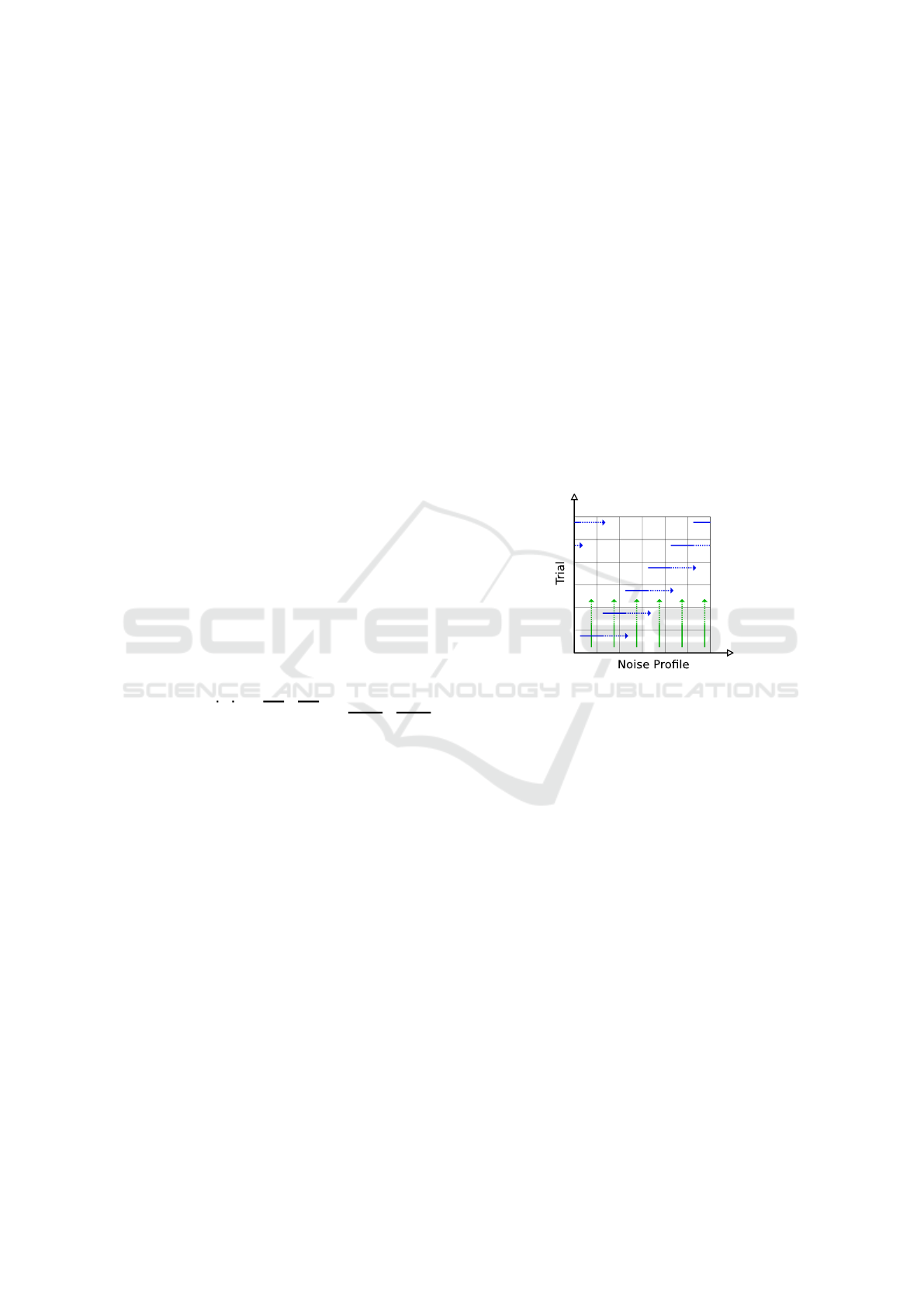
under fixed i.i.d. noise-profiles each. We propose a
method (see Figure 1) for re-using one set of sub-
models for both configurations. In this way we re-
duce the overall number of models we need to train.
Furthermore, by combining the same models in differ-
ent ways the difference between the same-noise con-
dition and the cross-noise condition is less affected
by model variability and mainly results from the en-
semble construction strategy. We combine the sub-
models for the cross-noise profile setting following
the cyclical pattern depicted in Figure 1. We do so in
order to minimize the effect of individual noise pro-
files on the average of measures over the ensembles.
If we choose the number of distinct noise-profiles to
be equal to the number of trials per noise-profile and
sufficiently large, then we obtain an empirical fine-
grained decomposition of the variance-error based on
the different sources of randomness, i.e. data noise
and model-derivation randomness.
Figure 1: Configuration Design for Ensembling Strategy
Comparison. Cross-noise profile ensembles are constructed
following the horizontal arrows and same-noise profile en-
sembles following the vertical arrows.
The effective complexity of deep learning mod-
els depends on multiple parameters. Accordingly, we
visualize the DD on the test error along the model
width (model-wise DD) and the training epoch count
(epoch-wise DD) in Figure 2. The model width is a
factor in the number of convolutional channels used in
the hidden layers of the VGG11 (Simonyan and Zis-
serman, 2014) and ResNet18 (He et al., 2016) visual
classification models we consider in this paper. The
ensembles considered in Figure 2 are cross-noise pro-
file ensembles.
We compare different ensembling strategies and
ensemble mixing functions as well as comparable
non-ensemble architectures in order to be able to dis-
entangle the effects of design components on general-
ization and on DD mitigation. We compare:
1. Single sub-learners trained with and without label
noise.
2. Same-noise profile ensembles: Ensembles over
models all trained under the same label noise pro-
Reduction of Variance-related Error through Ensembling: Deep Double Descent and Out-of-Distribution Generalization
33

file. We use the following mixing techniques for
these ensembles:
(a) Learnable fully-connected bias-free linear en-
sembling with Softmax normalization. The
outputs of the sub-learners are fed through a
linear layer whose parameters are learned dur-
ing an additional training process. This addi-
tional training is subject to the same noise pro-
file that the sub-learners were subjected to.
(b) Arithmetic mean-based ensembling: The out-
puts for each category over all learners are
mixed according to: f
e
=
1
N
∑
N
n=1
f
n
(c) Geometric mean-based ensembling: The out-
puts for each category over all learners are
mixed according to: f
e
∝
N
q
∏
N
n=1
f
n
(d) Plurality vote-based ensembling: The category
that is the first choice of the largest number of
sub-learners is selected by the ensemble.
3. Cross-noise profile ensembles: Ensembles over
models each trained under a different noise pro-
file by using mixing techniques (b), (c) and (d).
4. Mono-Ensembles: Geometric mean-based ensem-
ble architectures trained as single models un-
der the same training configurations as the sub-
learners.
1
5. Large Networks: Networks of the same architec-
ture type as the sub-learners, but with a parameter
count as close as possible to multiples of the pa-
rameter count of the sub-learners and all training
configurations left equal.
We are also interested in the implications of the
underspecification-related performance penalty out-
of-sample. To that end, we also study the effect of
approximating the central tendency of learning pro-
cedures through ensembling on alternative datasets
for the same classification problem. In particular,
we test small ResNet18 classifiers that have been
trained on CIFAR-10 that lie close to (width 12) or
slightly beyond (width 26) the interpolation thresh-
old on CIFAR-10.1 (Recht et al., 2018), CIFAR-10.2
(Lu et al., 2020), and the set of images contained
in CINIC-10 (Darlow et al., 2018) that were adapted
from ImageNet (Russakovsky et al., 2015). CIFAR-
10.1 was designed to present almost no distribution
shift w.r.t. standard CIFAR-10, whereas both CIFAR-
10.2 and CINIC-10 were constructed to realize differ-
ent data-distributions, e.g. regarding low level image
statistics and the sub-categories (i.e. synonym sets)
used for populating the classes.
Additional information on model training and ex-
1
During training, sub-network outputs passed on to the
ensembling layer where saturated to be greater or equal to
10
−5
. This prevents not-a-number errors.
perimental design along with further results is avail-
able in Rath-Manakidis (2021).
4 RESULTS
In this section we present the results of our experi-
ments and describe their implications.
4.1 Findings on Double Descent
We observed no DD without noise on CIFAR-10.
With almost no explicit regularization and without la-
bel noise, we obtained no epoch-wise DD on CIFAR-
10 for neither ResNet18 nor VGG11 models. There-
fore it is not possible in this case to empirically sep-
arate distinct learning regimes because the test error
exhibits a global monotonous trend.
Under most configurations tested, we obtained
epoch-wise DD w.r.t. the test set only w.r.t. the er-
ror and not the loss (see Plots 2b and 2c). This is
surprising given the fact that it is the loss that the net-
works were trained to minimize and that it is merely
intended as a proxy for the error that can be used
in back-propagation
2
, whereas in most other settings
(e.g. in regression) the measure used in optimization
itself exhibits DD on the test set. The test error is
the metric we ultimately intend to minimize and the
network is never confronted with it directly. For ex-
ample, in Plot 2c we see that the loss does not display
epoch-wise DD for this configuration and that it gen-
erally remains high, when compared to the values of
its first descent. Nevertheless, the error performs a
combined epoch-wise and model-wise DD. The loss
does perform a weak model-wise DD for large epoch
values but it does not reach again the values at the
bottom of the first valley of its trajectory.
The valley in Plot 2b for the test error DD curve
coincides with the valley of the noise-free train set
error in 2a. This implies that the test error ascend is
partly due to learning to fit label noise and is not a
phenomenon tied strictly to generalization.
We find that ensembling of deep networks, es-
pecially if realized through a geometric mean-based
approach to model output mixing, significantly im-
proves model performance (see Figures 3 and 4). We
attribute this to the capacity of the geometric-mean
ensemble to differentiate between strong and weak
preference for or against each category by the sub-
models: if some models weakly favor one category
2
E.g. the loss criterion is such that even correctly clas-
sified training inputs keep contributing to the optimization
signal to the network parameters.
ICPRAM 2022 - 11th International Conference on Pattern Recognition Applications and Methods
34
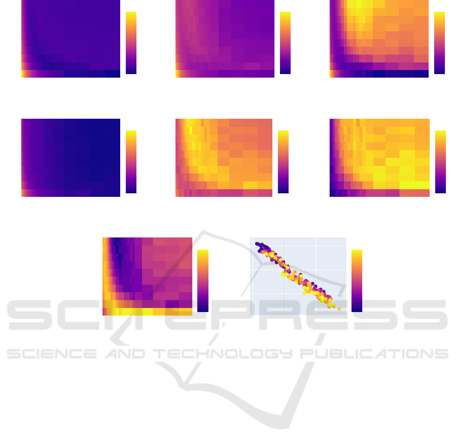
20 40 60
50
100
150
200
250
300
0.1
0.2
0.3
Error
Width
Epoch
(a) Error on the noise-free training set.
20 40 60
50
100
150
200
250
300
0.1
0.2
0.3
Error
Width
Epoch
(b) Test error.
20 40 60
50
100
150
200
250
300
0.6
0.8
1
Loss
Width
Epoch
(c) Test loss.
20 40 60
50
100
150
200
250
300
0.1
0.2
0.3
Error
Width
Epoch
(d) Ensemble test error.
20 40 60
50
100
150
200
250
300
0
0.02
0.04
0.06
0.08
Error
Width
Epoch
(e) Test error difference.
20 40 60
50
100
150
200
250
300
20
30
40
50
%
Width
Epoch
(f) Relative test error reduction.
20 40 60
50
100
150
200
250
300
0.8
0.85
0.9
Correlation
Width
Epoch
(g) Output correlation.
0.04 0.06 0.08
0.8
0.85
0.9
0
100
200
300
Epoch
Error Difference
Avg. Correlation
(h) Accuracy increase against correla-
tion.
Figure 2: Test error of ResNet18 on CIFAR-10. For each model-width and epoch combination we have rendered we ensemble
4 models with i.i.d. 10% label noise.
but a smaller number of models strongly prefer some
other category, the latter option may still be preferred
by the ensemble.
We find that those models that fall into the region
of the interpolation threshold of the DD phenomenon
profit most strongly from ensembling (see Plot 2e
here and Figure 28 in Nakkiran et al., 2019). They do
so in absolute and not in relative terms (cf. Plot 2f) in
accordance with the interpretation that the benefits of
ensembling hinge on the variability between the mod-
els. The observed performance improvement, at least
for the case where it depends on the existence of la-
bel noise, can be realized by using same-noise pro-
file ensembles almost as thoroughly as by cross-noise
profile ensembles (see e.g. Figure 5). It also turns out
that the generalization performance benefit of using
cross-noise profile ensembles over same-noise profile
ensembles tends to be statistically significant but quite
small in magnitude. This means that around the DD
hike most error variance of the learning procedure is
accounted for by the network weight initialization and
training-time randomness and only a small fraction
of the variance can be additionally explained away in
terms of the variation in the training noise profile. For
ML deployment, this implies that artifacts in the train-
ing data that enter during data acquisition (i.e. that
give rise to errors that constitute a noise profile) re-
sult, to a limited extend, in artifacts that cancel each
other out in the learned function mappings.
We proceed to present some observations from the
model type comparison in Figures 3 and 4. The ge-
ometric mean-based ensembler consistently outper-
forms all other ensembling methods, both with same-
noise profile and cross-noise profile sub-learners for
all ensemble sizes tested. We presume this is because
geometric mean-based ensembling utilizes the avail-
able information better than the other two static ap-
proaches we tested: arithmetic mean-based ensem-
bling fails to sufficiently reduce the impact of the
votes of models that weakly prefer some output cat-
Reduction of Variance-related Error through Ensembling: Deep Double Descent and Out-of-Distribution Generalization
35
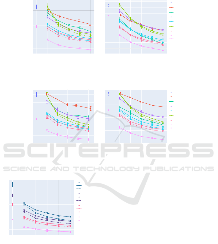
1 2 3 4 5 6
0.14
0.16
0.18
0.2
0.22
0.24
0.26
Sub Net
Big Net
MonoEnsemble
Fully Conn. Ens.
Eq. W. Ens.
Cross Eq. W. Ens.
Plurality Ens.
Cross Plurality Ens.
Geom. Ens.
Cross Geom. Ens.
0% Noise Sub Net
0% Noise Geom. Ens.
#SubNets
Error
(a) CIFAR-10, sub-model width 9.
1 2 3 4 5 6
0.4
0.42
0.44
0.46
0.48
0.5
0.52
0.54
Sub Net
Big Net
Mono-Ensemble
Fully Conn. Ens.
Arithm. Ens.
Plurality Ens.
Geom. Ens.
0% Noise Sub Net
0% Noise Geom. Ens.
#SubNets
Error
(b) CIFAR-100, sub-model width 11.
Figure 3: Test error of model trials based on VGG11. Continuous lines represent same-noise profile ensembles and dashed
lines cross-noise profile ensembles. Noise strength is 10% for CIFAR-10 and 5% for CIFAR-100. The setups are explained
in Section 3.
2 4 6
0.1
0.12
0.14
0.16
0.18
0.2
Sub Net
Big Net
Mono-Ensemble
Fully Conn. Ens.
Arithm. Ens.
Plurality Ens.
Geom. Ens.
0% Noise Sub Net
0% Noise Geom. Ens.
#SubNets
Error
(a) CIFAR-10, sub-model width 10.
1 2 3 4 5 6
0.35
0.4
0.45
Sub Net
Big Net
Mono-Ensemble
Fully Conn. Ens.
Arithm. Ens.
Plurality Ens.
Geom. Ens.
0% Noise Sub Net
0% Noise Geom. Ens.
#SubNets
Error
(b) CIFAR-100, sub-model width 11.
Figure 4: Test error of model trials based on ResNet18. Continuous lines represent same-noise profile ensembles and dashed
lines cross-noise profile ensembles. Noise strength is 10%.
1 2 3 4 5 6
0.1
0.15
0.2
0.25
0.3
30% Noise Sub Net
30% Same Noise Ens.
30% Cross Noise Ens.
20% Noise Sub Net
20% Same Noise Ens.
20% Cross Noise Ens.
10% Noise Sub Net
10% Same Noise Ens.
10% Cross Noise Ens.
0% Noise Sub Net
0% Noise Ens.
#SubNets
Error
Figure 5: Test error of ResNet18 on CIFAR-10, model
width 10. Continuous lines represent same-noise profile
ensembles and dashed lines cross-noise profile ensembles.
The colors code for noise strength.
egory over the others and plurality vote-based en-
sembling abstracts from any information regarding
weak preference or strong rejection of categories. The
additional training for the ensembles with a fully-
connected linear layer as ensembling layer is less ca-
pable of facilitating generalization. The error back-
propagation is conducted based on the error of the en-
semble prediction rather than the errors of the pre-
dictions of the constituent modules for the mono-
ensemble architecture. This architecture performs
mostly worse than architecturally identical ensembles
and better than monolithic architectures with equiva-
lent parameter count.
With our experimental results we support the
suggestion made by Geiger et al. (2020) that “. . . ,
given a computational envelope, the smallest gen-
eralization error is obtained using several networks
of intermediate sizes, just beyond N
∗
, and averag-
ing their outputs”, under slightly more realistic con-
ditions, whereby N
∗
refers to the interpolation thresh-
old model parameterization. In Table 1 we show that
a given computational envelope can be utilized more
effectively if we train for a given type of model archi-
tecture many same-noise profile networks around the
interpolation threshold in parallel and combine them
for deployment, instead of training a large single net-
work. In this way we require fewer computational
steps for training and fewer parameters in total.
ICPRAM 2022 - 11th International Conference on Pattern Recognition Applications and Methods
36

Table 1: Relative performance of ensembles and full-width
networks for ResNet18 on CIFAR-10. The models were
trained on 10% label noise and the ensembles are same-
noise ensembles of 6 sub-learners. Models with widths 10
and 12 are interpolation threshold models. The mean per-
formance of the ensembles of the models of width 10 and
12 is statistically significantly different from that of the full-
width networks judging by the standard error of the mean.
Sub-model
#Parameters
Test Error
Width Mean ± SEM
6 597696 0.1304 ± 0.00082
10 1649880 0.1162 ± 0.00084
12 2372100 0.1123 ± 0.00048
26 11088696 0.0919 ± 0.00058
Single net
Width
64 11173962 0.1307 ± 0.00180
4.2 Interpretation of Relative Model
Performance
In those experiments where we have estimated the av-
erage performance of geometric mean-based ensem-
bles, mono-ensembles and large networks (Figures 3
and 4), we see the general pattern that large networks
perform worse than mono-ensembles which in turn
tend to perform worse than geometric mean ensem-
bles of the same-noise profile type.
3
We conjecture
that this trend is due to internal correlations between
the components (e.g. layers and channels) in some of
the models. Table 1 shows that ensembles of models
at the interpolation threshold can perform well while
using relatively little memory. We attribute this to
the good accuracy of their mean prediction and to the
low degree of output correlation between these mod-
els (see Figures 2g and 2e) which permits extensive
variance reduction through model averaging. We plot
the accuracy increase due to ensembling against the
strength of the correlations between the models con-
stituting the ensemble in Plot 2h.
Geometric mean-based ensembles tend to perform
better than comparable mono-ensembles (see e.g. Fig-
ure 3a). The latter differ from the former in that there
is a shared last layer and that they are being trained
through back-propagation on the loss of their overall
predictions. Additionally, mono-ensembles face less
diverse data shuffling and augmentation during train-
ing.
4
3
With the exception of the experiment reported in Fig-
ure 3b where mono-ensembles outperform all regular en-
sembles.
4
The input to each sub-module in the mono-ensemble
for each training batch was always identical: it was not sub-
Because of the two above-mentioned factors, dur-
ing training there are identical influences on the
sub-modules and the loss signal each sub-module is
trained on is not specific to the individual module’s
divergence from the ground truth. This, in turn, may
introduce correlations between the sub-modules, in
the sense that it couples their training trajectories and
causes the model as a whole to learn a less diverse and
differentiated set of hidden features.
The worst performance in our comparison among
models with an almost identical parameter count was
that of large single networks. This can be attributed
to the fact that the intermediary results of the compu-
tations in these models are used more often than in
the other models. This leads to internal correlations
between the parameters within the hidden layers of
these models during back-propagation: In the large
networks the number of parameters corresponding to
each computational element (e.g. convolution chan-
nel) is larger than in the ensemble architectures and
the internal state of the networks is more compact,
i.e. fewer variables are used for storing intermediate
results during forward-propagation. This impairs iso-
lating relevant structure in the hidden features.
4.3 In-Distribution and
Out-of-Distribution Generalization
For a given architecture, e.g. ResNet18 models of
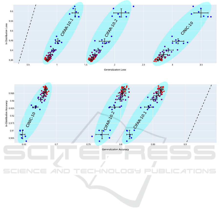
width 12 (Figure 6) or width 26 (Figure 7), the loss
of the ensembles correlates linearly between differ-
ent test sets as the number of sub-networks in the en-
sembles changes (cf. Miller et al., 2021). Likewise,
a linear correlation also exists between the accuracy
values on the different test sets. We also observe,
as expected, that with increasing ensemble size the
generalization performance increases and converges
toward a limit. Simultaneously, the variance in the
performance between distinct ensembles diminishes.
We observe these trends for all transfer test sets we
experimented on, regardless of the extend of distribu-
tion shift. This implies that the in-distribution bene-
fit of ensembling predicts its out-of-distribution utility
well. The increase in test-set performance by forming
small ensembles can be used to estimate whether or
not training further sub-models in order to form even
larger ensembles is a worthwhile strategy for repre-
senting the meaningful structure of the problem at
hand.
ject to independent selection and augmentation as was the
case for the regular ensembles. This was necessary to reli-
ably train all parameters using one loss signal.
Reduction of Variance-related Error through Ensembling: Deep Double Descent and Out-of-Distribution Generalization
37
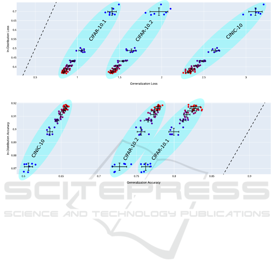
(a) Loss
(b) Accuracy
Figure 6: ResNet18 on CIFAR-10, model width 12. Blue points represent single models and red points ensembles of 7 models.
Intermediary colors represent ensembles of sizes 2 to 6. We do not use label noise.
5 DISCUSSION
In this paper we present further examples of the
DD generalization curve of the error on classifica-
tion problems. Although we demonstrate a non-
monotonous trend of the error for a range of up to
now untested conditions and also approximate a bias-
variance-decomposition of the error, the question in
as far this is the same phenomenon that has been anal-
ysed in shallow models (e.g. Belkin et al., 2019; Ad-
vani et al., 2020; Mei and Montanari, 2019) remains
open, because of the way loss and error relate and the
fact that the trend of the error often contradicts that of
its corresponding loss. This divergence is especially
strong at and beyond the interpolation threshold and it
raises the question in as far one could use alternative
learning objectives to reliably mitigate the DD hike
(cf. Ishida et al., 2020). We illustrate this divergence
in Section 4.1 where we present results for deep learn-
ing settings for which certain types of DD occur only
for the error and not for the loss.
In Table 1 we present the finding that small mod-
els that individually are impaired by DD can afford
ensembles that outperform single large models while
requiring considerably fewer overall parameters and
computational steps. This has practical implications
because it shows, that allowing for more intricate
models with more complicated hidden features is not
always the best approach to augment model perfor-
mance if the model design suffers from underspecifi-
cation. In particular, with a sufficiently general and
reliable ensemble definition (geometric-mean ensem-
bling) and with model and training procedure defi-
nitions that contain impactful sources of randomness
we demonstrate how multiple predictors can be com-
bined through ensembling to produce a considerably
better model. This is the case even if we do not com-
bine multiple learner types or strategies and without
access to noise-free training data. The performance
improvement through same-noise profile ensembling
was on par with the improvement gained when also
redrawing the noise on the training data (see Figure
5).
In Section 4.2 we propose an interpretation of the
model architecture comparison in terms of coupled
ICPRAM 2022 - 11th International Conference on Pattern Recognition Applications and Methods
38
(a) Loss
(b) Accuracy
Figure 7: ResNet18 on CIFAR-10, model width 26. Same legend as for Figure 6.
training dynamics and ensuing model correlation that
we hope will be scrutinized in future research. Fu-
ture research is also needed to verify the degree of
validity of the notion of error decomposition for clas-
sification problems and to mathematically ground the
notion of a distribution of mappings and its evolution
in the course of training.
With our out-of-distribution generalization exper-
iments in Section 4.3 we show that the general trend
of in-distribution generalization of increasingly large
ensembles applies also to out-of-distribution settings
and that the beneficial effects of ensembling general-
ize beyond the training distribution in a regular man-
ner.
REFERENCES
Adlam, B. and Pennington, J. (2020a). The neural tangent
kernel in high dimensions: Triple descent and a multi-
scale theory of generalization. In International Con-
ference on Machine Learning, pages 74–84. PMLR.
Adlam, B. and Pennington, J. (2020b). Understanding dou-
ble descent requires a fine-grained bias-variance de-
composition.
Advani, M. S., Saxe, A. M., and Sompolinsky, H. (2020).
High-dimensional dynamics of generalization error in
neural networks. Neural Networks, 132:428 – 446.
Belkin, M., Hsu, D., Ma, S., and Mandal, S. (2019). Recon-
ciling modern machine-learning practice and the clas-
sical bias–variance trade-off. Proceedings of the Na-
tional Academy of Sciences, 116(32):15849–15854.
Belkin, M., Ma, S., and Mandal, S. (2018). To understand
deep learning we need to understand kernel learn-
ing. In International Conference on Machine Learn-
ing, pages 541–549. PMLR.
Chen, L., Min, Y., Belkin, M., and Karbasi, A. (2020). Mul-
tiple descent: Design your own generalization curve.
arXiv preprint arXiv:2008.01036.
D’Amour, A., Heller, K., Moldovan, D., Adlam, B., Ali-
panahi, B., Beutel, A., Chen, C., Deaton, J., Eisen-
stein, J., Hoffman, M. D., Hormozdiari, F., Houlsby,
N., Hou, S., Jerfel, G., Karthikesalingam, A., Lucic,
M., Ma, Y., McLean, C., Mincu, D., Mitani, A., Mon-
tanari, A., Nado, Z., Natarajan, V., Nielson, C., Os-
borne, T. F., Raman, R., Ramasamy, K., Sayres, R.,
Schrouff, J., Seneviratne, M., Sequeira, S., Suresh,
H., Veitch, V., Vladymyrov, M., Wang, X., Webster,
K., Yadlowsky, S., Yun, T., Zhai, X., and Sculley,
D. (2020). Underspecification presents challenges
Reduction of Variance-related Error through Ensembling: Deep Double Descent and Out-of-Distribution Generalization
39

for credibility in modern machine learning. arXiv
preprint arXiv:2011.03395.
Darlow, L. N., Crowley, E. J., Antoniou, A., and Storkey,
A. J. (2018). CINIC-10 is not ImageNet or CIFAR-
10. arXiv preprint arXiv:1810.03505.
d’Ascoli, S., Refinetti, M., Biroli, G., and Krzakala, F.
(2020). Double trouble in double descent: Bias and
variance (s) in the lazy regime. In International
Conference on Machine Learning, pages 2280–2290.
PMLR.
Geiger, M., Jacot, A., Spigler, S., Gabriel, F., Sagun, L.,
d’Ascoli, S., Biroli, G., Hongler, C., and Wyart, M.
(2020). Scaling description of generalization with
number of parameters in deep learning. Journal
of Statistical Mechanics: Theory and Experiment,
2020(2):023401.
He, K., Zhang, X., Ren, S., and Sun, J. (2016). Deep resid-
ual learning for image recognition. In Proceedings of
the IEEE conference on computer vision and pattern
recognition, pages 770–778.
Ishida, T., Yamane, I., Sakai, T., Niu, G., and Sugiyama, M.
(2020). Do we need zero training loss after achieving
zero training error? In International Conference on
Machine Learning, pages 4604–4614. PMLR.
Jacot, A., Gabriel, F., and Hongler, C. (2018). Neural tan-
gent kernel: convergence and generalization in neu-
ral networks. In Proceedings of the 32nd Interna-
tional Conference on Neural Information Processing
Systems, pages 8580–8589.
Lakshminarayanan, B., Pritzel, A., and Blundell, C. (2017).
Simple and scalable predictive uncertainty estimation
using deep ensembles. Advances in Neural Informa-
tion Processing Systems, pages 6402–6413.
Lee, J., Bahri, Y., Novak, R., Schoenholz, S. S., Penning-
ton, J., and Sohl-Dickstein, J. (2017). Deep neu-
ral networks as gaussian processes. arXiv preprint
arXiv:1711.00165.
Lu, S., Nott, B., Olson, A., Todeschini, A., Vahabi, H., Car-
mon, Y., and Schmidt, L. (2020). Harder or different?
a closer look at distribution shift in dataset reproduc-
tion. In ICML Workshop on Uncertainty and Robust-
ness in Deep Learning.
Mei, S. and Montanari, A. (2019). The generalization er-
ror of random features regression: Precise asymp-
totics and double descent curve. arXiv preprint
arXiv:1908.05355.
Miller, J. P., Taori, R., Raghunathan, A., Sagawa, S.,
Koh, P. W., Shankar, V., Liang, P., Carmon, Y., and
Schmidt, L. (2021). Accuracy on the line: on the
strong correlation between out-of-distribution and in-
distribution generalization. In International Confer-
ence on Machine Learning, pages 7721–7735. PMLR.
Nakkiran, P., Kaplun, G., Bansal, Y., Yang, T., Barak, B.,
and Sutskever, I. (2019). Deep double descent: Where
bigger models and more data hurt. arXiv preprint
arXiv:1912.02292.
Opper, M., Kinzel, W., Kleinz, J., and Nehl, R. (1990).
On the ability of the optimal perceptron to gener-
alise. Journal of Physics A: Mathematical and Gen-
eral, 23(11):L581.
Rasmussen, C. E. (2003). Gaussian processes in machine
learning. In Summer school on machine learning,
pages 63–71. Springer.
Rath-Manakidis, P. (2021). Interaction of ensembling and
double descent in deep neural networks. Master’s the-
sis, Cognitive Science, Ruhr University Bochum, Ger-
many.
Recht, B., Roelofs, R., Schmidt, L., and Shankar, V. (2018).
Do CIFAR-10 classifiers generalize to CIFAR-10?
arXiv preprint arXiv:1806.00451.
Russakovsky, O., Deng, J., Su, H., Krause, J., Satheesh, S.,
Ma, S., Huang, Z., Karpathy, A., Khosla, A., Bern-
stein, M., et al. (2015). Imagenet large scale visual
recognition challenge. International journal of com-
puter vision, 115(3):211–252.
Simonyan, K. and Zisserman, A. (2014). Very deep con-
volutional networks for large-scale image recognition.
arXiv preprint arXiv:1409.1556.
Yang, Z., Yu, Y., You, C., Steinhardt, J., and Ma, Y. (2020).
Rethinking bias-variance trade-off for generalization
of neural networks. In International Conference on
Machine Learning, pages 10767–10777. PMLR.
ICPRAM 2022 - 11th International Conference on Pattern Recognition Applications and Methods
40
