
DenseHMM: Learning Hidden Markov Models by Learning Dense
Representations
Joachim Sicking
1,2
, Maximilian Pintz
1,3
, Maram Akila
1
and Tim Wirtz
1,2
1
Fraunhofer IAIS, Sankt Augustin, Germany
2
Fraunhofer Center for Machine Learning, Sankt Augustin, Germany
3
University of Bonn, Bonn, Germany
Keywords:
Hidden Markov Model, Representation Learning, Gradient Descent Optimization.
Abstract:
We propose DenseHMM – a modification of Hidden Markov Models (HMMs) that allows to learn dense
representations of both the hidden states and the (discrete) observables. Compared to the standard HMM,
transition probabilities are not atomic but composed of these representations via kernelization. Our approach
enables constraint-free and gradient-based optimization. We propose two optimization schemes that make use
of this: a modification of the Baum-Welch algorithm and a direct co-occurrence optimization. The latter one is
highly scalable and comes empirically without loss of performance compared to standard HMMs. We show
that the non-linearity of the kernelization is crucial for the expressiveness of the representations. The properties
of the DenseHMM like learned co-occurrences and log-likelihoods are studied empirically on synthetic and
biomedical datasets.
1 INTRODUCTION
Hidden Markov Models (Rabiner and Juang, 1986)
have been a state-of-the-art approach for modelling
sequential data for more than three decades (Hin-
ton et al., 2012). Their success story is proven by
a large number of applications ranging from natural
language modelling (Chen and Goodman, 1999) and
automatic speech recognition (Bahl et al., 1986; Varga
and Moore, 1990) over financial services (Bhusari and
Patil, 2016) to robotics (Fu et al., 2016). While still be-
ing used frequently, many more recent approaches are
based on neural networks instead, like feed-forward
neural networks (Schmidhuber, 2015), recurrent neu-
ral networks (Hochreiter and Schmidhuber, 1997) or
spiked neural networks (Tavanaei et al., 2019). How-
ever, the recent breakthroughs in the field of neural
networks (LeCun et al., 2015; Schmidhuber, 2015;
Goodfellow et al., 2016; Minar and Naher, 2018; Deng
et al., 2013; Paul et al., 2015; Wu et al., 2020) are
accompanied by an almost equally big lack of their
theoretical understanding. In contrast, HMMs come
with a broad theoretical understanding, for instance
of the parameter estimation (Yang et al., 2017), con-
vergence (Wu, 1983; Dempster et al., 1977), con-
sistency (Leroux, 1992) and short-term prediction
performance (Sharan et al., 2018), despite of their
non-convex optimization landscape.
Different from HMMs, (neural) representa-
tion learning became more prominent only re-
cently (Mikolov et al., 2013b; Pennington et al., 2014).
From the very first day following their release, ap-
proaches like word2vec or Glove (Mikolov et al.,
2013b; Pennington et al., 2014; Mikolov et al., 2013a;
Le and Mikolov, 2014) that yield dense representations
for state sequences, have significantly emphasized the
value of pre-trained representations of discrete sequen-
tial data for downstream tasks (Kim, 2014; Wang et al.,
2019). Since then those found application not only
in language modeling (Mikolov et al., 2013c; Zhang
et al., 2016b; Li and Yang, 2018; Almeida and Xexéo,
2019) but also in biology (Asgari and Mofrad, 2015;
Zou et al., 2019), graph analysis (Perozzi et al., 2014;
Grover and Leskovec, 2016) and even banking (Bal-
dassini and Serrano, 2018). Similar approaches have
received an overwhelming attention and became part
of the respective state-of-the-art approaches.
Ever since, the quality of representation models
increased steadily, driven especially by the natural
language community. Recently, so-called transformer
networks (Vaswani et al., 2017) were put forward, com-
plex deep architectures that leverage attention mecha-
nisms (Bahdanau et al., 2015; Kim et al., 2017). Their
complexity and tremendously large amounts of com-
Sicking, J., Pintz, M., Akila, M. and Wirtz, T.
DenseHMM: Learning Hidden Markov Models by Learning Dense Representations.
DOI: 10.5220/0010821800003122
In Proceedings of the 11th International Conference on Pattern Recognition Applications and Methods (ICPRAM 2022), pages 237-248
ISBN: 978-989-758-549-4; ISSN: 2184-4313
Copyright
c
2022 by SCITEPRESS – Science and Technology Publications, Lda. All rights reserved
237

pute and training data lead again to remarkable im-
provements on a multitude of natural language pro-
cessing (NLP) tasks (Devlin et al., 2019).
These developments are particularly driven by the
question on how to optimally embed discrete sequences
into a continuous space. However, many existing ap-
proaches identify optimality solely with performance
and put less emphasize on aspects like conceptual sim-
plicity and theoretical soundness. Intensified discus-
sions on well-understood and therefore trustworthy
machine learning (Saltzer and Schroeder, 1975; Dwork
et al., 2012; Amodei et al., 2016; Gu et al., 2017;
Varshney, 2019; Toreini et al., 2020; Brundage et al.,
2020) indicate, however, that these latter aspects be-
come more and more crucial or even mandatory for
real-world learning systems. This holds especially true
when representing biological structures and systems
as derived insights may be used in downstream appli-
cations, e.g. of medical nature where physical harm
can occur.
In light of this, we propose DenseHMM – a modi-
fication of Hidden Markov Models that allows to learn
dense representations of both the hidden states and
the discrete observables
(Figure 1)
. Compared to the
standard HMM, transition probabilities are not atomic
but composed of these representations. Concretely, we
contribute
•
a parameter-efficient, non-linear matrix factoriza-
tion for HMMs,
•
two competitive approaches to optimize the result-
ing DenseHMM
•
and an empirical study of its performance and prop-
erties on diverse datasets.
The rest of the work is organized as follows: first,
we present related work on HMM parameter learn-
ing and matrix-factorization approaches in section 2.
Next, DenseHMM and its optimization schemes are
introduced in section 3. We study the effect of its soft-
max non-linearity and conduct empirical analyses and
comparisons with standard HMMs in sections 4 and 5,
respectively. A discussion in section 6 concludes our
paper.
2 RELATED WORK
HMMs are generative models with Markov proper-
ties for sequences of either discrete or continuous ob-
servation symbols (Rabiner, 1989). They assume a
number of non-observable (hidden) states that drive
the dynamics of the generated sequences. If domain
expertise allows to interpret these drivers, HMMs can
be fully understood. This distinguishes HMMs from
sequence-modelling neural networks like long short-
term memory networks (Hochreiter and Schmidhuber,
1997) and temporal convolutional networks (Bai et al.,
2018). More recent latent variable models that keep
the discrete structure of the latent space make use of,
e.g., Indian buffet processes (Griffiths and Ghahra-
mani, 2011). These allow to dynamically adapt the
dimension of the latent space dependent on data com-
plexity and thus afford more flexible modelling. While
we stay in the HMM model class, we argue that our
approach allows to extend or reduce the latent space in
a more principled way compared to standard HMMs.
Various approaches exist to learn the parameters of
hidden Markov models: A classical one is the Baum-
Welch algorithm (Rabiner, 1989) that handles the com-
plexity of the joint likelihood of hidden states and
observables by introducing an iterative two-step pro-
cedure that makes use of the forward-backward al-
gorithm (Rabiner and Juang, 1986). Another algo-
rithm for (local) likelihood maximization is (Baldi and
Chauvin, 1994). The authors of (Huang et al., 2018)
study HMM learning on observation co-occurrences
instead of observation sequences. Based on moments,
i.e. co- and triple-occurrences, bounds on the em-
pirical probabilities can be derived via spectral de-
composition (Anandkumar et al., 2012). Approaches
from Bayesian data analysis comprise Markov chain
Monte Carlo (MCMC) and variational
inference (VI)
.
While MCMC can provide more stable and better re-
sults (Rybert Sipos, 2016), it traditionally suffers from
poor scalability. A more scalable stochastic-gradient
MCMC algorithm that tackles mini-batching of se-
quentially dependent data is (Ma et al., 2017). The
same authors propose a stochastic VI (SVI) algorithm
(Foti et al., 2014) that shares some technical details
with (Ma et al., 2017). SVI for hierarchical Dirich-
let process (HDP) HMMs is considered in (Zhang
et al., 2016a). For our DenseHMM, we adapt two
non-Bayesian procedures: the Baum-Welch algorithm
(Rabiner, 1989) and direct co-occurrence optimization
(Huang et al., 2018). The latter we optimize, solely
for convenience, using a deep learning framework.
1
In (Tran et al., 2016) this idea was carried further, al-
lowing different modifications to the original HMM
context. Already earlier, combinations of HMMs and
neural networks were employed, for instance for auto-
matic speech recognition (Bourlard et al., 1992; Moon
and Hwang, 1997; Trentin and Gori, 1999).
Non-negative matrix factorization (NMF, (Lee and
Seung, 1999)) splits a matrix into a pair of low-rank
matrices with solely positive components. NMF for
HMM learning is used, e.g., in (Lakshminarayanan
and Raich, 2010; Cybenko and Crespi, 2011). In
1
See appendix C for details.
ICPRAM 2022 - 11th International Conference on Pattern Recognition Applications and Methods
238
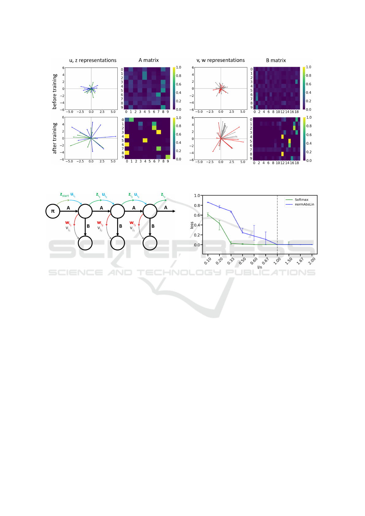
Figure 1: Exemplary DenseHMM to visualize the inner workings of our approach. All model components are shown before
(top row) and after training (bottom row). The transition matrices
A
(second column) and
B
(fourth column) are learned by
learning dense representations (first and third column). All representations are initialized by a standard Gaussian.
Figure 2: Structure of the DenseHMM. The HMM parame-
ters A,
B
and
π
are composed of vector representations such
that A = A(U, Z), B = B(V,W) and π = π(U,z
start
).
contrast, we combine matrix factorization with a non-
linear kernel function to ensure non-negativity and
normalization of the HMM transition matrices. Fur-
ther foci of recent work on HMMs are identifiability
(Huang et al., 2018), i.e. uniqueness guarantees for an
obtained model, and optimized priors over transition
distributions (Qiao et al., 2015).
3 STRUCTURE AND
OPTIMIZATION OF THE DENSE
HMM
A HMM is defined by two time-discrete stochastic pro-
cesses:
{X
t
}
t∈N
is a Markov chain over hidden states
S = {s
i
}
n
i=1
and
{Y
t
}
t∈N
is a process over observable
states
O = {o
i
}
m
i=1
. The central assumption of HMMs
is that the probability to observe
Y
t
= y
t
depends only
on the current state of the hidden process and the
probability to find
X
t
= x
t
only on the the previous
state of the hidden process,
X
t−1
= x
t−1
for all
t ∈ N
.
We denote the state-transition matrix as
A ∈ R
n×n
Figure 3: Approximation quality of non-linear matrix fac-
torizations. The optimization errors (median, 25/75 per-
centile) of softmax (green) and normAbsLin (blue) matrices
are shown over the ratio of representation length
l
and matrix
size n. The vertical line indicates l = n.
with
a
i j
= P(X
t
= s
j
| X
t−1
= s
i
)
, the emission matrix
as
B ∈ R
n×m
with
b
i j
= P(Y
t
= o
j
| X
t
= s
i
)
and the
initial state distribution as
π ∈ R
n
with
π
i
= P(X
1
= s
i
)
.
A HMM is fully parametrized by λ = (A,B,π).
HMMs can be seen as extensions of Markov chains
(MCs) which are in turn closely related to word2vec
embeddings. Let us elaborate on this: A MC has
no hidden states and is defined by just one process
{X
t
}
t∈N
over observables. The transition dynamics of
the states of the MC is described by a transition ma-
trix
A
and an initial distribution
π
. Being in a given
state
s
I
, the MC models conditional probabilities of
the form
p(s
i
| s
I
)
. MCs are structurally similar to
the approaches that learn word2vec representations,
i.e. continuous bag of words and skip-gram (Mikolov
et al., 2013b). Both models learn transitions between
the words of a text corpus. Each word
w
i
of the vocab-
ulary is represented by a learned dense vector
u
i
. The
transition probabilities between words are recovered
DenseHMM: Learning Hidden Markov Models by Learning Dense Representations
239

from the scalar products of these vectors:
p(w
j
| w
i
) =
exp(u
i
· v
j
)
∑
k
exp(u
i
· v
k
)
∝ exp(u
i
· v
j
). (1)
The learned word2vec representations are low-
dimensional and context-based, i.e. they contain se-
mantic information. This is in contrast to the trivial
and high-dimensional one-hot (or bag-of-word) encod-
ings.
Here we transfer the non-linear factorization ap-
proach of word2vec (eq. 1) to HMMs. This is done
by composing
A,B
and
π
of dense vector representa-
tions such that
a
i j
= a
i j
(U,Z) =
exp(u
j
· z
i
)
∑
k∈[n]
exp(u
k
· z
i
)
, (2a)
b
ik
= b
ik
(V,W) =
exp(v
k
· w
i
)
∑
k
′
∈[m]
exp(v
k
′
· w
i
)
, (2b)
π
i
= π
i
(U,z
start
) =
exp(u
i
· z
start
)
∑
k∈[n]
exp(u
k
· z
start
)
, (2c)
for
i, j ∈ [n]
and
k ∈ [m]
. Let us motivate this transfor-
mation (Fig. 2) piece by piece: each representation
vector corresponds to either a hidden state (
u
i
,
w
i
,
z
i
)
or an observation (
v
i
). The vector
u
i
(
z
i
) is the incom-
ing (outgoing) representation of hidden state
i
along
the (hidden) Markov chain.
w
i
is the outgoing rep-
resentation of hidden state
i
towards the observation
symbols. These are described by the
v
i
. All vectors
are real-valued and of length
l
.
A
and
B
each depend
on two kinds of representations instead of only one to
enable non-symmetric transition matrices. Addition-
ally, to choose
A
independent of
B
, as is typical for
HMMs, we need
w
i
as a third hidden representation. It
is convenient to summarize all representation vectors
of one kind in a matrix (U , V ,W , Z).
A softmax kernel maps the scalar products of the
representations onto the HMM parameters
A,B
and
π
. Softmax maps to the simplex and thus ensures
a
i j
,
b
i j
,
π
i
to be in
[0,1]
as well as row-wise normalization
of
A
,
B
and
π
. While a different kernel function
may be chosen, a strong non-linearity, such as in the
softmax kernel, is essential to obtain matrices
A
and
B
with high ranks (compare experiments in section
4).
This non-linear kernelization enables constraint-
free optimization which is a central property of our
approach. We use this fact in two different ways:
we derive a modified expectation-maximization (EM)
scheme in section 3.1 and study an alternative to
EM optimization that is based on co-occurrences in
section 3.2.
3.1
EM Optimization: a Gradient-based
M-step
We briefly recapitulate the EM-based Baum-Welch
algorithm (Bishop, 2007) and adapt it to learn the
proposed representations as part of the M-step:
Given a sequence
o
of length
T ∈ N
over observa-
tions
O
, the Baum-Welch algorithm finds parameters
λ
that (locally) maximize the observation likelihoods.
A latent distribution
Q
over the hidden states
S
is intro-
duced such that the log-likelihood of the sequence
decomposes as follows:
L(Q,λ) = logP(o,λ) =
L(Q,λ) + KL(Q||P(· | o, λ))
.
KL(P||Q)
de-
notes the Kullback-Leibler divergence from
Q
to
P
with
P,Q
being probability distributions and
L(Q,λ) =
∑
x∈S
T
Q(x)log [P(x, o;λ)/Q(x)]
. Start-
ing from an initial guess for
λ
, the algorithm alternates
between two sub-procedures, the E- and M-step: In
the E-step, the forward-backward algorithm (Bishop,
2007) is used to update
Q = P(· | o; λ)
, which maxi-
mizes
L(Q,λ)
for fixed
λ
. The efficient computation
of the conditional probabilities
γ
t
(s,s
′
) := P(X
t−1
=
s,X
t
= s
′
| o)
and
γ
t
(s) := P(X
t
= s | o)
for
s,s
′
∈ S
is
crucial for the E-step. In the M-step, the latent distribu-
tion
Q
is fixed and
L(Q,λ)
is maximized w.r.t.
λ
under
normalization constraints. As the Kullback-Leibler di-
vergence
KL
is set to zero in each E-step, the function
to maximize in the M-step becomes
L(Q,λ) =
∑
x∈S
T
Q(x)log
P(x,o; λ)
Q(x)
=
∑
x∈S
T
P(x | o; λ
old
)log
P(x,o; λ)
P(x | o; λ
old
)
with
λ
old
being the parameter obtained in the previous
M-step. Applying the logarithm to
P(x,o; λ)
, which
has a product structure due to the Markov properties,
splits the optimization objective into three summands.
Each term depends on only one of the parameters
A,B, π:
A
∗
,B
∗
,π
∗
= arg max
A,B,π
L(Q,λ)
=arg max
A,B,π
L
1
(Q,A) + L
2
(Q,B) + L
3
(Q,π).
Due to structural similarities between the three sum-
mands, we consider only
L
1
in the following. The
treatment of
L
2
and
L
3
can be found in appendix A.
For L
1
, we have
L
1
(Q,A) =
∑
i∈[n]
T
P(s
i
| o; λ
old
)
T
∑
t=2
log(a
i
t−1
,i
t
)
with multi-index
s
i
= s
i
1
,...,s
i
T
. The next step is to re-
write
L
1
in terms of
γ
t
and to use Lagrange multipliers
ICPRAM 2022 - 11th International Conference on Pattern Recognition Applications and Methods
240

to ensure normalization. This gives the following part
¯
L
1
of the full Lagrangian
¯
L =
¯
L
1
+
¯
L
2
+
¯
L
3
:
¯
L
1
:=
∑
i, j∈[n]
T
∑
t=2
γ
t
(s
i
,s
j
)log a
i j
+
∑
i∈[n]
ϕ
i
1 −
∑
j∈[n]
a
i j
with Lagrange multipliers
ϕ
i
for each
i ∈ [n]
to ensure
that A is a proper transition matrix.
To optimize DenseHMM, we leave the E-step
unchanged and modify the M-step by applying the
parametrization of
λ
, i.e. equations (2a)-(2c), to the
Lagrangian
¯
L
. Please note that we can drop all nor-
malization constraints as they are explicitly enforced
by the softmax function. This turns the original con-
strained optimization problem of the M-step into an
unconstrained one, leading to a Lagrangian of the form
¯
L
dense
=
¯
L
dense
1
+
¯
L
dense
2
+
¯
L
dense
3
with
¯
L
dense
1
=
∑
i, j∈[n]
T
∑
t=2
γ
t
(s
i
,s
j
)u
j
· z
i
−
∑
i, j∈[n]
T
∑
t=2
γ
t
(s
i
,s
j
)log
∑
k∈[n]
exp(u
k
· z
i
).
We optimize
¯
L
dense
with gradient-decent procedures
such as SGD (Bottou, 2010) and Adam (Kingma and
Ba, 2015).
3.2 Direct Optimization of Observation
Co-occurrences: Gradient-based and
Scalable
Inspired by (Huang et al., 2018), we investigate an
alternative to the EM scheme: directly optimizing
co-occurrence probabilities. The ground truth co-
occurrences
Ω
gt
are obtained from training data
o
by calculating the relative frequencies of subsequent
pairs
(o
i
(t),o
j
(t + 1)) ∈ O
2
. If we know that
o
is gen-
erated by a HMM with a stationary hidden process,
we can easily compute
Ω
gt
analytically as follows:
we summarize all co-occurrence probabilities
Ω
i j
=
P(Y
t
= o
i
,Y
t+1
= o
j
)
for
i, j ∈ [m]
in a co-occurrence
matrix
Ω = B
T
ΘB
with
Θ
kl
= P(X
t
= s
k
,X
t+1
= s
l
)
for
k, l ∈ [n]
. We can further write
Θ
kl
= P(X
t+1
=
s
l
| X
t
= s
k
)P(X
t
= s
k
) = A
kl
π
k
for
i, j ∈ [n]
under the
assumption that
π
is the stationary distribution of
A
,
i.e.
π
j
=
∑
i
A
i j
π
i
for all
i, j ∈ [n]
. Then, we obtain the
co-occurrence probabilities
Ω
i j
=
∑
k,l∈[n]
π
k
b
ki
a
kl
b
l j
for i, j ∈ [m]. (3)
Parametrizing the matrices
A
and
B
according to eq.
(2a,2b) yields
Ω
dense
i j
(U , V ,W , Z)
=
∑
k,l∈[n]
π
k
b
ki
(V,W)a
kl
(U,Z)b
l j
(V,W)
for
i, j ∈ [m]
. Please note that
π
is not parametrized
here. Following our stationarity demand it is chosen as
the eigenvector v
λ=1
of
A
T
. We minimize the squared
distance between
Ω
dense
and
Ω
gt
w.r.t. the vector rep-
resentations, i.e.
argmin
U ,V ,W ,Z
||Ω
gt
− Ω
dense
(U , V ,W , Z)||
2
F
,
using gradient-decent procedures like SGD and Adam.
4 PROPERTIES OF THE DENSE
HMM
To further motivate our approach, please note that a
standard HMM with
n
hidden states and
m
observa-
tion symbols has
n
2
+ n(m − 1) − 1
degrees of free-
dom (DOFs), whereas a DenseHMM with represen-
tation length
l
has
l(3n + m + 1)
DOFs. Therefore,
a low-dimensional representation length
l
leads to
DenseHMMs with less DOFs compared to a standard
HMM for many values of
n
and
m
. A linear factoriza-
tion with representation length
l < n
leads to rank
l
for the matrices
A
and
B
, whereas a non-linear factor-
ization can yield more expressive full rank matrices.
This effect of non-linearities may be best understood
with a simple toy example: assume a 2x2 matrix with
co-linear columns:
[[1,2],[2, 4]]
. Applying a softmax
column-wise leads to a matrix
∝ [[e,e
2
],C[e
2
,e
4
]]
with
linearly independent columns. More general, the soft-
max rescales and rotates each column of
U Z
and
V W
differently and (except for special cases) thus
increases the matrix rank to full rank. It is worth to
mention that any other kernel
k : R
l
× R
l
→ R
+
could
be used instead of exp in the softmax to recover the
HMM parameters from the representations, e.g. sig-
moid, ReLU or RBFs.
As non-linear matrix factorization is a central
building block of our approach, we compare the
approximation quality of softmax with an appropriate
linear factorization in the following setup: we generate
a Dirichlet-distributed ground truth matrix
A
gt
∈ R
n×n
and approximate it (i) by
˜
A = softmax(UZ)
defined
by
softmax(UZ)
ij
= exp
(UZ)
ij
/
∑
k
exp((UZ)
ik
)
and (ii) by a normalized absolute matrix
product
˜
A = normAbsLin(UZ)
defined by
normAbsLin(UZ)
ij
= |(UZ)
ij
|/
∑
k
|(UZ)
ik
|
. Note
that we report the resulting error
||
˜
A − A
gt
||
F
divided
by
||A
gt
||
F
to get comparable losses independent of
the size of
A
gt
. These optimizations are performed
for matrix sizes
n = 3,5, 10
, several representation
lengths
l
and
10
different
A
gt
for each
(n,l)
pair.
Table 1 in appendix A provides all considered
(n,l)
pairs and detailed results. Fig. 3 shows that the
softmax non-linearity yields closer approximations of
DenseHMM: Learning Hidden Markov Models by Learning Dense Representations
241

A
gt
compared to normAbsLin. Moreover, we observe
on a qualitative level significantly faster convergence
for softmax as
l
increases. For softmax, vector lengths
l ≈ n/3
suffice to closely fit
A
gt
while the piece-wise
linear normAbsLin requires
l = n
. This result is in
accordance with our remarks above.
5 EMPIRICAL EVALUATION
We investigate the outlined optimization schemes
w.r.t. obtained model quality and behaviors. We com-
pare the following types of models:
H
EM
dense
:
a DenseHMM optimized with the EM
optimization scheme (section 3.1),
H
direct
dense
:
a DenseHMM optimized with direct op-
timization of co-occurrences (section
3.2),
H
stand
:
a standard HMM optimized with
the Baum-Welch algorithm (Rabiner,
1989).
These models all have the same number of hidden
states
n
and observation symbols
m
. If a standard
HMM and a DenseHMM use the same
n
and
m
, one of
the models may have less DOFs than the other (cp. sec-
tion 4). Therefore, we also consider the model
H
fair
stand
,
which is a standard HMM with a similar amount of
DOFs compared to a given
H
dense
model. We denote
the number of hidden states in
H
fair
stand
as
n
fair
, which
is the positive solution of
n
2
fair
+ n
fair
(m − 1) − 1 =
l(3n +m + 1)
rounded to the nearest integer. Note that
n
fair
can get significantly larger than
n
for
l > n
and
therefore
H
fair
stand
is expected to outperform the other
models in these cases.
We use two standard measures to assess
model quality: the co-occurrence mean absolute
deviation (MAD)
and the normalized negative log-
likelihood (NLL). The MAD between two co-
occurrence matrices
Ω
gt
and
Ω
model
is defined as
1/m
2
∑
i, j∈[m]
|Ω
model
i j
− Ω
gt
i j
|
. We compute both
Ω
gt
and
Ω
model
based on sufficiently long sampled se-
quences (more details in appendix C). In the case
of synthetically generated ground truth sequences,
we compute
Ω
gt
analytically instead. In addition,
we take a look at the negative log-likelihood of the
ground truth test sequences
{o
test
i
}
under the model,
i.e.
NLL = −
∑
i
logP(o
test
i
;λ)
. We conduct experi-
ments with
n ∈ {3,5, 10}
and different representation
lengths
l
for each
n
. For each
(n,l)
combination, we
run
10
experiments with different train-test splits. We
evaluate the median and 25/75 percentiles of the co-
occurrence MADs and the normalized NLLs for each
of the four models (see appendix C for details).
In the following, we consider synthetically gener-
ated data as well as two real-world datasets: amino
acid sequences from the RCSB PDB dataset (Berman
et al., 2000) and part-of-speech tag sequences of
biomedical text (Smith et al., 2004), referred to as
the MedPost dataset.
Synthetic Sequences. We sample training and test
ground truth sequences from a standard HMM
H
syn
that is constructed as follows: Each row of the tran-
sition matrices
A
and
B
is drawn from a Dirichlet
distribution
Dir(α)
, where all entries in
α
are set to
a fixed value
α = 0.1
. The initial state distribution
π
is set to the normalized eigenvector
v
λ=1
of
A
T
. This
renders
H
syn
stationary and allows a simple analytical
calculation of
Ω
gt
according to eq. 3. For both training
and testing, we sample
10
sequences, each of length
200
with
m = n
emission symbols. Figure 4 left shows
our evaluation w.r.t. co-occurrence MADs. Note that
the performance of
H
stand
changes slightly with
l
for
fixed
n
as training is performed on different sequences
for every
(n,l)
pair. This is because the sequences
are re-drawn from
H
syn
for every experiment. The
standard HMMs and
H
direct
dense
perform similarly, with
H
direct
dense
performing slightly better throughout the ex-
periments and especially for
n = 3
.
H
EM
dense
shows a
higher MAD than the other models. The good perfor-
mance of
H
direct
dense
may be explained by the fact that it
optimizes a function similar to co-occurrence MADs,
whereas the other models aim to optimize negative log-
likelihoods. The results in Figure 4 right show that the
DenseHMMs reach comparable NLLs, although the
standard HMMs perform slightly better in this metric.
Proteins. The RCSB PDB dataset (Berman et al.,
2000) consists of
512,145
amino acid sequences from
which we only take the first
1,024
. After applying
preprocessing (described in further detail in appendix
C), we randomly shuffle the sequences and split train
and test data 50:50 for each experiment. Figure 5 left
shows the results of our evaluation w.r.t. co-occurrence
MADs.
H
EM
dense
performs slightly worse than both
H
stand
and
H
fair
stand
. We observe that
H
direct
dense
yields the
best results. While the co-occurrence MADs of
H
EM
dense
,
H
stand
and
H
fair
stand
stay roughly constant throughout
different experiments,
H
direct
dense
can utilize larger
n
and
l
to further decrease co-occurrence MADs. As can be
seen in Figure 5 right, all models achieve almost identi-
cal normalized NLLs throughout the experiments. The
results suggest that model size has only a minor im-
pact on normalized NLL performance for the protein
dataset.
ICPRAM 2022 - 11th International Conference on Pattern Recognition Applications and Methods
242
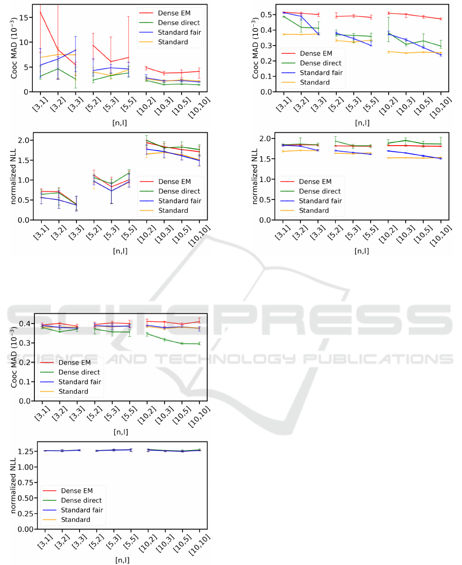
Figure 4: Co-occurrence mean absolute deviation (left) and
normalized negative log-likelihood (right) of the models
H
EM
dense
,
H
direct
dense
,
H
fair
stand
,
H
stand
on synthetically generated
sequences evaluated for multiple combinations of n and l.
Figure 5: Co-occurrence mean absolute deviation (left) and
normalized negative log-likelihood (right) of the models
H
EM
dense
,
H
direct
dense
,
H
fair
stand
,
H
stand
on amino acid sequences
evaluated for multiple combinations of n and l.
Part-of-Speech Sequences. The MedPost dataset
(Smith et al., 2004) consists of
5,700
sentences. Each
Figure 6: Co-occurrence mean absolute deviation (left) and
normalized negative log-likelihood (right) of the models
H
EM
dense
,
H
direct
dense
,
H
fair
stand
,
H
stand
on part-of-speech tag se-
quences (Medpost) evaluated for multiple combinations of
n
and l.
sentence consists of words that are tagged with one of
60
part-of-speech items. Sequences of part-of-speech
tags are considered such that each sequence corre-
sponds to one sentence. We apply preprocessing sim-
ilar to the protein dataset (more details in appendix
C). The sequences are randomly shuffled and train and
test data is split 50:50 for each experiment. Figure
6 left shows performance of our models in terms of
co-occurrence MADs. We see that the performance
of the standard HMM models as well as
H
direct
dense
in-
creases with increasing
n
. The number of hidden states
seems to be a major driver of performance. Accord-
ingly,
H
fair
stand
improves with growing
n
fair
(l) ∝ l
. Plus,
we have
n
fair
> n
for
l ≈ n
which fully explains why
H
fair
stand
is the best performing model in these cases.
Overall,
H
direct
dense
performs competitive to
H
fair
stand
, es-
pecially for the practically more relevant cases with
l < n
. Similar to the other datasets,
H
EM
dense
performs
worse than the other models and is barely affected by
increasing
n
. Both DenseHMM models have increas-
ing performance for increasing
l
. Normalized NLLs
(Figure 6 right) are best for the standard HMM models.
Both DenseHMM models achieve similar normalized
NLLs, which are slightly worse than the ones achieved
by the standard HMM models.
DenseHMM: Learning Hidden Markov Models by Learning Dense Representations
243

6 DISCUSSION
We learn hidden Markov models by learning dense,
real-valued vector representations for its hidden and
observable states. The involved softmax non-linearity
enables to learn high-rank transition matrices, i.e. pre-
vents that the matrix ranks are immediately determined
by the chosen (in most cases) low-dimensional repre-
sentation length. We successfully optimize our models
in two different ways and find direct co-occurrence
optimization to yield competitive results compared to
the standard HMM. This optimization technique re-
quires only one gradient descent procedure and no
iterative multi-step schemes. It is highly scalable with
training data size and also with model size - as it is
implemented in a modern deep-learning framework.
The optimization is stable and does neither require
fine-tuning of learning rate nor of the representation
initializations. We release our full tensorflow code to
foster active use of DenseHMM in the community.
We leave it to future work to adapt DenseHMMs to
HMMs with continuous emissions and study variants
of DenseHMM with fewer kinds of learnable repre-
sentations. First experiments with DenseHMMs that
learn only
Z
and
V
lead to almost comparable model
quality. From a practitioner’s viewpoint, it is worth
to investigate how DenseHMM and the learned repre-
sentations perform on downstream tasks. Using the
MedPost dataset, one could consider part-of-speech
labeling of word sequences via the Viterbi algorithm
after identifying the hidden states of the model with
a pre-defined set of ground truth tags. For the protein
dataset, a comparison with LSTM-based and BERT
embeddings (Bepler and Berger, 2019; Min et al.,
2019) could help to understand similarities and dif-
ferences resulting from modern representation learn-
ing techniques. An analysis of geometrical proper-
ties of the learned representations seems promising
for systems with
l ≫ 1
as
exp(l)
many vectors can
be almost-orthogonal in
R
l
. The
V
representations
are a natural choice for such a study as they directly
correspond to observation items. The integration of
Bayesian optimization techniques like MCMC and VI
with DenseHMM is another research avenue.
ACKNOWLEDGEMENTS
The research of J. Sicking and T. Wirtz was funded by
the Fraunhofer Center for Machine Learning within
the Fraunhofer Cluster for Cognitive Internet Tech-
nologies. The work of M. Pintz and M. Akila was
funded by the German Federal Ministry of Education
and Research, ML2R - no. 01S18038B. The authors
thank Jasmin Brandt for fruitful discussions.
REFERENCES
Abadi, M., Barham, P., Chen, J., Chen, Z., Davis, A., Dean,
J., Devin, M., Ghemawat, S., Irving, G., Isard, M., et al.
(2016). Tensorflow: A system for large-scale machine
learning. In 12th USENIX Symposium on Operating
Systems Design and Implementation, pages 265–283.
Almeida, F. and Xexéo, G. (2019). Word embeddings: A
survey. arXiv preprint arXiv:1901.09069.
Amodei, D., Olah, C., Steinhardt, J., Christiano, P., Schul-
man, J., and Mané, D. (2016). Concrete problems in
AI safety. arXiv preprint arXiv:1606.06565.
Anandkumar, A., Hsu, D. J., and Kakade, S. M. (2012).
A method of moments for mixture models and hid-
den Markov models. In Mannor, S., Srebro, N., and
Williamson, R. C., editors, COLT 2012 - The 25th
Annual Conference on Learning Theory, June 25-27,
2012, Edinburgh, Scotland, volume 23 of JMLR Pro-
ceedings, pages 33.1–33.34. JMLR.org.
Asgari, E. and Mofrad, M. R. (2015). Continuous distributed
representation of biological sequences for deep pro-
teomics and genomics. PloS One, 10(11):e0141287.
Bahdanau, D., Cho, K., and Bengio, Y. (2015). Neural
machine translation by jointly learning to align and
translate. In Bengio, Y. and LeCun, Y., editors, 3rd
International Conference on Learning Representations,
ICLR 2015, San Diego, CA, USA, May 7-9, 2015, Con-
ference Track Proceedings.
Bahl, L., Brown, P., De Souza, P., and Mercer, R. (1986).
Maximum mutual information estimation of hidden
Markov model parameters for speech recognition. In
ICASSP’86. IEEE International Conference on Acous-
tics, Speech, and Signal Processing, volume 11, pages
49–52. IEEE.
Bai, S., Kolter, J. Z., and Koltun, V. (2018). An empir-
ical evaluation of generic convolutional and recur-
rent networks for sequence modeling. arXiv preprint
arXiv:1803.01271.
Baldassini, L. and Serrano, J. A. R. (2018). client2vec:
towards systematic baselines for banking applications.
arXiv preprint arXiv:1802.04198.
Baldi, P. and Chauvin, Y. (1994). Smooth on-line learning
algorithms for hidden Markov models. Neural Compu-
tation, 6(2):307–318.
Bepler, T. and Berger, B. (2019). Learning protein sequence
embeddings using information from structure. In 7th
International Conference on Learning Representations,
ICLR 2019, New Orleans, LA, USA, May 6-9, 2019.
Berman, H. M., Westbrook, J., Feng, Z., Gilliland, G., Bhat,
T. N., Weissig, H., Shindyalov, I. N., and Bourne, P. E.
(2000). The protein data bank. Nucleic acids research,
28(1):235–242.
Bhusari, V. and Patil, S. (2016). Study of hidden Markov
model in credit card fraudulent detection. In 2016
World Conference on Futuristic Trends in Research
and Innovation for Social Welfare (Startup Conclave),
ICPRAM 2022 - 11th International Conference on Pattern Recognition Applications and Methods
244

pages 1–4. IEEE.
Bishop, C. M. (2007). Pattern Recognition and Ma-
chine Learning (Information Science and Statistics).
Springer, 1 edition.
Bottou, L. (2010). Large-scale machine learning with
stochastic gradient descent. In Proceedings of COMP-
STAT’2010, pages 177–186. Springer.
Bourlard, H., Morgan, N., and Renals, S. (1992). Neural
nets and hidden Markov models: Review and general-
izations. Speech Communication, 11(2-3):237–246.
Brundage, M., Avin, S., Wang, J., Belfield, H., Krueger, G.,
Hadfield, G., Khlaaf, H., Yang, J., Toner, H., Fong,
R., et al. (2020). Toward trustworthy AI development:
Mechanisms for supporting verifiable claims. arXiv
preprint arXiv:2004.07213.
Chen, S. F. and Goodman, J. (1999). An empirical study of
smoothing techniques for language modeling. Com-
puter Speech & Language, 13(4):359–394.
Cybenko, G. and Crespi, V. (2011). Learning hidden
Markov models using nonnegative matrix factorization.
IEEE Transactions on Information Theory, 57(6):3963–
3970.
Dempster, A. P., Laird, N. M., and Rubin, D. B. (1977).
Maximum likelihood from incomplete data via the EM
algorithm. Journal of the Royal Statistical Society:
Series B (Methodological), 39(1):1–22.
Deng, L., Li, J., Huang, J.-T., Yao, K., Yu, D., Seide, F.,
Seltzer, M., Zweig, G., He, X., Williams, J., et al.
(2013). Recent advances in deep learning for speech
research at Microsoft. In 2013 IEEE International Con-
ference on Acoustics, Speech and Signal Processing,
pages 8604–8608. IEEE.
Devlin, J., Chang, M., Lee, K., and Toutanova, K. (2019).
BERT: pre-training of deep bidirectional transformers
for language understanding. In Burstein, J., Doran,
C., and Solorio, T., editors, Proceedings of the 2019
Conference of the North American Chapter of the As-
sociation for Computational Linguistics: Human Lan-
guage Technologies, NAACL-HLT 2019, Minneapolis,
MN, USA, June 2-7, 2019, Volume 1 (Long and Short
Papers), pages 4171–4186. Association for Computa-
tional Linguistics.
Dwork, C., Hardt, M., Pitassi, T., Reingold, O., and Zemel,
R. (2012). Fairness through awareness. In Proceedings
of the 3rd Innovations in Theoretical Computer Science
Conference, pages 214–226.
Foti, N., Xu, J., Laird, D., and Fox, E. (2014). Stochastic
variational inference for hidden Markov models. In
Advances in Neural Information Processing Systems,
pages 3599–3607.
Fu, R., Wang, H., and Zhao, W. (2016). Dynamic driver
fatigue detection using hidden Markov model in real
driving condition. Expert Systems with Applications,
63:397–411.
Goodfellow, I., Bengio, Y., and Courville, A. (2016). Deep
learning. MIT press.
Griffiths, T. L. and Ghahramani, Z. (2011). The Indian
buffet process: An introduction and review. Journal of
Machine Learning Research, 12(Apr):1185–1224.
Grover, A. and Leskovec, J. (2016). node2vec: Scalable fea-
ture learning for networks. In Proceedings of the 22nd
ACM SIGKDD International Conference on Knowl-
edge Discovery and Data Mining, pages 855–864.
ACM.
Gu, T., Dolan-Gavitt, B., and Garg, S. (2017). Badnets: Iden-
tifying vulnerabilities in the machine learning model
supply chain. arXiv preprint arXiv:1708.06733.
Hinton, G., Deng, L., Yu, D., Dahl, G. E., Mohamed, A.-
r., Jaitly, N., Senior, A., Vanhoucke, V., Nguyen, P.,
Sainath, T. N., et al. (2012). Deep neural networks for
acoustic modeling in speech recognition: The shared
views of four research groups. IEEE Signal Processing
Magazine, 29(6):82–97.
Hochreiter, S. and Schmidhuber, J. (1997). Long short-term
memory. Neural Computation, 9(8):1735–1780.
Huang, K., Fu, X., and Sidiropoulos, N. (2018). Learning
hidden Markov models from pairwise co-occurrences
with application to topic modeling. In Proceedings of
the 35th International Conference on Machine Learn-
ing, pages 2068–2077. PMLR.
Kim, Y. (2014). Convolutional neural networks for sentence
classification. In Proceedings of the 2014 Conference
on Empirical Methods in Natural Language Processing
(EMNLP), pages 1746–1751, Doha, Qatar. Association
for Computational Linguistics.
Kim, Y., Denton, C., Hoang, L., and Rush, A. M. (2017).
Structured attention networks. In 5th International
Conference on Learning Representations, ICLR 2017,
Toulon, France, April 24-26, 2017, Conference Track
Proceedings. OpenReview.net.
Kingma, D. P. and Ba, J. (2015). Adam: A method for
stochastic optimization. In Bengio, Y. and LeCun,
Y., editors, 3rd International Conference on Learning
Representations, ICLR 2015, San Diego, CA, USA,
May 7-9, 2015, Conference Track Proceedings.
Lakshminarayanan, B. and Raich, R. (2010). Non-negative
matrix factorization for parameter estimation in hidden
Markov models. In 2010 IEEE International Workshop
on Machine Learning for Signal Processing, pages 89–
94. IEEE.
Le, Q. and Mikolov, T. (2014). Distributed representations of
sentences and documents. In International Conference
on Machine Learning, pages 1188–1196.
LeCun, Y., Bengio, Y., and Hinton, G. (2015). Deep learning.
Nature, 521(7553):436–444.
Lee, D. D. and Seung, H. S. (1999). Learning the parts of
objects by non-negative matrix factorization. Nature,
401(6755):788–791.
Leroux, B. G. (1992). Maximum-likelihood estimation for
hidden Markov models. Stochastic Processes and their
Applications, 40(1):127–143.
Li, Y. and Yang, T. (2018). Word embedding for understand-
ing natural language: a survey. In Guide to Big Data
Applications, pages 83–104. Springer.
Ma, Y.-A., Foti, N. J., and Fox, E. B. (2017). Stochastic
gradient MCMC methods for hidden Markov models.
In Proceedings of the 34th International Conference
on Machine Learning-Volume 70, pages 2265–2274.
JMLR. org.
DenseHMM: Learning Hidden Markov Models by Learning Dense Representations
245

Mikolov, T., Chen, K., Corrado, G., and Dean, J. (2013a).
Efficient estimation of word representations in vector
space. In Bengio, Y. and LeCun, Y., editors, 1st In-
ternational Conference on Learning Representations,
ICLR 2013, Scottsdale, Arizona, USA, May 2-4, 2013,
Workshop Track Proceedings.
Mikolov, T., Sutskever, I., Chen, K., Corrado, G. S., and
Dean, J. (2013b). Distributed representations of words
and phrases and their compositionality. In Advances in
Neural Information Processing Systems, pages 3111–
3119.
Mikolov, T., Yih, W.-t., and Zweig, G. (2013c). Linguistic
regularities in continuous space word representations.
In Proceedings of the 2013 Conference of the North
American Chapter of the Association For Computa-
tional Linguistics: Human Language Technologies,
pages 746–751.
Min, S., Park, S., Kim, S., Choi, H.-S., and Yoon, S. (2019).
Pre-training of deep bidirectional protein sequence rep-
resentations with structural information. Neural In-
formation Processing Systems, Workshop on Learning
Meaningful Representations of Life.
Minar, M. R. and Naher, J. (2018). Recent advances
in deep learning: An overview. arXiv preprint
arXiv:1807.08169.
Moon, S. and Hwang, J.-N. (1997). Robust speech recogni-
tion based on joint model and feature space optimiza-
tion of hidden Markov models. IEEE Transactions on
Neural Networks, 8(2):194–204.
Paul, S., Singh, L., et al. (2015). A review on advances in
deep learning. In 2015 IEEE Workshop on Computa-
tional Intelligence: Theories, Applications and Future
Directions (WCI), pages 1–6. IEEE.
Pennington, J., Socher, R., and Manning, C. (2014). Glove:
Global vectors for word representation. In Proceedings
of the 2014 Conference on Empirical Methods in Natu-
ral Language Processing (EMNLP), pages 1532–1543.
Perozzi, B., Al-Rfou, R., and Skiena, S. (2014). Deep-
walk: Online learning of social representations. In
Proceedings of the 20th ACM SIGKDD International
Conference on Knowledge Discovery and Data Mining,
pages 701–710. ACM.
Qiao, M., Bian, W., Da Xu, R. Y., and Tao, D. (2015). Diver-
sified hidden Markov models for sequential labeling.
IEEE Transactions on Knowledge and Data Engineer-
ing, 27(11):2947–2960.
Rabiner, L. R. (1989). A tutorial on hidden Markov models
and selected applications in speech recognition. Pro-
ceedings of the IEEE, 77(2):257–286.
Rabiner, L. R. and Juang, B.-H. (1986). An introduction to
hidden Markov models. IEEE ASSP Magazine, 3(1):4–
16.
Rybert Sipos, I. (2016). Parallel stratified MCMC sampling
of AR-HMMs for stochastic time series prediction. In
Proceedings of the 4th Stochastic Modeling Techniques
and Data Analysis International Conference with De-
mographics Workshop (SMTDA 2016). Valletta, Malta:
University of Malta, pages 361–364.
Saltzer, J. H. and Schroeder, M. D. (1975). The protection
of information in computer systems. Proceedings of
the IEEE, 63(9):1278–1308.
Schmidhuber, J. (2015). Deep learning in neural networks:
An overview. Neural Networks, 61:85–117.
Sharan, V., Kakade, S., Liang, P., and Valiant, G. (2018).
Prediction with a short memory. In Proceedings of the
50th Annual ACM SIGACT Symposium on Theory of
Computing, pages 1074–1087. ACM.
Smith, L., Rindflesch, T., and Wilbur, W. J. (2004). MedPost:
a part-of-speech tagger for bioMedical text. Bioinfor-
matics, 20(14):2320–2321.
Tavanaei, A., Ghodrati, M., Kheradpisheh, S. R., Masquelier,
T., and Maida, A. (2019). Deep learning in spiking
neural networks. Neural Networks, 111:47–63.
Toreini, E., Aitken, M., Coopamootoo, K., Elliott, K., Zelaya,
C. G., and van Moorsel, A. (2020). The relationship
between trust in AI and trustworthy machine learning
technologies. In Proceedings of the 2020 Conference
on Fairness, Accountability, and Transparency, pages
272–283.
Tran, K. M., Bisk, Y., Vaswani, A., Marcu, D., and Knight, K.
(2016). Unsupervised neural hidden Markov models.
In SPNLP@EMNLP, pages 63–71.
Trentin, E. and Gori, M. (1999). Combining neural networks
and hidden Markov models for speech recognition.
Neural Nets WIRN VIETRI-98, pages 63–79.
Varga, A. and Moore, R. K. (1990). Hidden Markov model
decomposition of speech and noise. In International
Conference on Acoustics, Speech, and Signal Process-
ing, pages 845–848. IEEE.
Varshney, K. R. (2019). Trustworthy machine learning and
artificial intelligence. XRDS: Crossroads, The ACM
Magazine for Students, 25(3):26–29.
Vaswani, A., Shazeer, N., Parmar, N., Uszkoreit, J., Jones,
L., Gomez, A. N., Kaiser, Ł., and Polosukhin, I. (2017).
Attention is all you need. In Advances in Neural Infor-
mation Processing Systems, pages 5998–6008.
Wang, B., Wang, A., Chen, F., Wang, Y., and Kuo, C.-C. J.
(2019). Evaluating word embedding models: Meth-
ods and experimental results. APSIPA transactions on
signal and information processing, 8.
Wu, C. J. (1983). On the convergence properties of the EM
algorithm. The Annals of Statistics, pages 95–103.
Wu, X., Sahoo, D., and Hoi, S. C. (2020). Recent advances
in deep learning for object detection. Neurocomputing.
Yang, F., Balakrishnan, S., and Wainwright, M. J. (2017).
Statistical and computational guarantees for the Baum-
Welch algorithm. The Journal of Machine Learning
Research, 18(1):4528–4580.
Zhang, A., Gultekin, S., and Paisley, J. (2016a). Stochastic
variational inference for the HDP-HMM. In Artificial
Intelligence and Statistics, pages 800–808.
Zhang, Y., Rahman, M. M., Braylan, A., Dang, B., Chang,
H., Kim, H., McNamara, Q., Angert, A., Banner, E.,
Khetan, V., McDonnell, T., Nguyen, A. T., Xu, D., Wal-
lace, B. C., and Lease, M. (2016b). Neural information
retrieval: A literature review. CoRR, abs/1611.06792.
Zou, Q., Xing, P., Wei, L., and Liu, B. (2019). Gene2vec:
gene subsequence embedding for prediction of mam-
malian N6-methyladenosine sites from mRNA. RNA,
25(2):205–218.
ICPRAM 2022 - 11th International Conference on Pattern Recognition Applications and Methods
246

APPENDIX
A Full Lagrangians of Standard
HMM and DenseHMM
The full Lagrangian of the standard HMM model in
the M-step reads
¯
L =
¯
L
1
+
¯
L
2
+
¯
L
3
=
∑
i, j∈[n]
T
∑
t=2
γ
t
(s
i
,s
j
)log a
i j
+
∑
i∈[n]
ϕ
i
1 −
∑
j∈[n]
a
i j
+
∑
i∈[n]
T
∑
t=1
γ
t
(s
i
)log b
i, j
o
t
+
∑
i∈[n]
ε
i
1 −
∑
j∈[m]
b
i j
+
∑
i∈[n]
γ
1
(s
i
)log π
i
+
¯
ϕ
1 −
∑
i∈[n]
π
i
,
where
j
o
t
describes the index of the observation ob-
served at time
t
and
¯
ϕ,ε
i
are Lagrange multipliers. Ap-
plying the transformations A
=
A
(
U, Z
)
, B
=
B
(
V,W
)
and
π = π(
U
,
z
start
)
yields the full Lagrangian of the
DenseHMM:
¯
L
dense
=
¯
L
dense
1
+
¯
L
dense
2
+
¯
L
dense
3
=
∑
i, j∈[n]
T
∑
t=2
γ
t
(s
i
,s
j
)u
j
· z
i
−
∑
i, j∈[n]
T
∑
t=2
γ
t
(s
i
,s
j
)log
∑
k∈[n]
exp(u
k
· z
i
)
+
∑
i∈[n]
T
∑
t=1
γ
t
(s
i
)v
j
o
t
· w
i
−
∑
i∈[n]
T
∑
t=1
γ
t
(s
i
)log
∑
j∈[m]
exp(v
j
· w
i
)
+
∑
i∈[n]
γ
1
(s
i
)u
i
· z
start
−
∑
i∈[n]
γ
1
(s
i
)log
∑
j∈[n]
exp(u
j
· z
start
).
B Non-linear A-Matrix Factorization
All matrix sizes
n
and representation lengths
l
that
contribute to the visualized
l/n
ratios in Figure 3 are
shown in Table 1.
C Implementation Details and Data
Preprocessing
Implementation Details. The backbone of our im-
plementation is the library
hmmlearn
2
that provides
functions to optimize and score HMMs. The optimiza-
tion schemes for the DenseHMM models
H
EM
dense
and
H
direct
dense
are implemented in tensorflow (Abadi et al.,
2016). Both models use
tf.train.AdamOptimizer
with a fixed learning rate for optimization. At this point
we note that experiments done with other optimizers
such that
tf.train.GradientDescentOptimizer
lead to similar results in the evaluation. The repre-
sentations are initialized using a standard isotropic
Gaussian distribution.
NLL
values are normalized by
the number of test sequences and by the maximum test
sequence length.
Hardware Used. All experiments are conducted
on a
Intel(R) Xeon(R) Silver 4116 CPU
with
2.10GHz and a NVidia Tesla V100.
Protein Dataset Preprocessing. The first
1,024
se-
quences of the RCSB PDB dataset have
22
unique
symbols. We cut each sequence after a length of
512
.
Note that less than
4.9%
of the
1,024
sequences ex-
ceed that length. Additionally, we collect the symbols
of lowest frequency that together make up less than
0.2%
of all symbols in the sequences and map them
onto one residual symbol. This reduces the number of
unique symbols in the sequences from 22 to 19.
Part-of-speech Sequences Preprocessing. We take
1,000
sequences from the Medpost dataset (from
tag_mb.ioc
) and cut them after a length of
40
which
affects less than
15%
of all sequences. We also collect
the tags of lowest frequency that together make up less
than
1%
of all tags in the sequences and map them
onto one residual tag. This reduces the number of tag
items from 60 to 42.
Calculation of
Ω
gt
and
Ω
Model
. The co-occurrence
matrices
Ω
model
and
Ω
gt
used to calculate the co-
occurrence MADs in section 5 are estimated by
counting subsequent pairs of observation symbols
(o
i
(t),o
j
(t + 1)) ∈ O
2
. For real-world data,
Ω
gt
is es-
timated based on the test data ground truth sequences.
Equally long sequences sampled from the trained
model are used to estimate
Ω
model
. In case of synthetic
data, Ω
gt
is calculated analytically (eq. 3) instead.
2
https://github.com/hmmlearn/hmmlearn
DenseHMM: Learning Hidden Markov Models by Learning Dense Representations
247

Table 1: Approximation errors (median with 25/75 percentile) of normAbsLin-based and softmax-based matrix factorizations
for different matrix sizes n and representation lengths l.
n l median (25/75 percentile) of loss(
˜
A,A
gt
)
˜
A = normAbsLin(UZ)
˜
A = softmax(UZ)
3 1 0.678 (0.652/0.696) 0.048 (0.004/0.110)
3 2 0.162 (0.002/0.270) 0.001 (0.000/0.001)
3 3 0.001 (0.001/0.001) 0.001 (0.000/0.001)
3 5 0.001 (0.001/0.001) 0.001 (0.001/0.001)
5 1 0.769 (0.745/0.827) 0.453 (0.321/0.505)
5 3 0.346 (0.093/0.396) 0.001 (0.001/0.003)
5 5 0.001 (0.001/0.002) 0.001 (0.001/0.001)
5 10 0.001 (0.001/0.002) 0.002 (0.001/0.003)
10 1 0.862 (0.851/0.868) 0.616 (0.581/0.645)
10 5 0.310 (0.235/0.345) 0.012 (0.005/0.028)
10 10 0.002 (0.002/0.002) 0.003 (0.002/0.005)
10 15 0.002 (0.002/0.002) 0.003 (0.003/0.043)
ICPRAM 2022 - 11th International Conference on Pattern Recognition Applications and Methods
248
