GAMS: Graph Augmentation with Module Swapping

Alessandro Bicciato and Andrea Torsello

Department of Environmental Sciences, Informatics and Statistics, Ca’ Foscari University of Venice, Italy

Keywords:

Augmentation, Motif, Swapping.

Abstract:

Data augmentation is a widely adopted approach to solve the large-data requirements of modern deep learning

techniques by generating new data instances from an existing dataset. While there is a huge literature and

experience on augmentation for vectorial or image-based data, there is relatively little work on graph-based

missing connectivity based on the original edge statistics and node similarity. We then test the performance

of the proposed augmentation approach against state-of-the-art approaches, showing that on datasets, where

the information is dominated by structure rather than node labels, we obtain a significant improvement with

respect to alternatives.

1 INTRODUCTION

Deep Learning techniques have proved to be effective

in tackling a wide range of real-world tasks due to

their ability to effectively learn low- to medium-level

representation for the problems at hand, and to pro-

vide more complex decision boundaries to reflect the

tion, i.e. the generation of new plausible that simu-

lates a re-sampling of the space of possible training

instances, by transforming and recombining the exist-

ing data. Augmentation operations are easily devised

for computer vision and natural language process-

ing tasks where one can express nuisance data trans-

formations that modify the input without modifying

the original semantic grouping. For example, object

translation and rotation, occlusion, and background

substitutions can readily be used on object detection

sity of the feature space. However, even continuity

Graphs have long been used as a powerful abstrac-

tion for a wide variety of real-world data where struc-

ture plays a key role, from collaborations (Lima et al.,

2014) to biological data (Gilmer et al., 2017; Ye et al.,

2015). While Graph Neural Networks (GNNs) have

gained increasing traction in the machine learning

community for being able to effectively tackle clas-

sification problem abstracted in terms of graphs, the

increased complexity of deep models expresses itself

in these approaches as well, resulting in a tendency to

that can be harder to come by than in the case of im-

ages and text, since graph-based representation reside

at a higher semantic level and cannot be acquired as

easily.

However, data augmentation techniques for

graphs is still under-researched, with most methods

performing simple node and edge edit operations

with little consideration of the larger structure of the

Bicciato, A. and Torsello, A.

GAMS: Graph Augmentation with Module Swapping.

graphs. In this paper we propose a novel augmenta-

tion approach called Graph Augmentation with Mod-

ule Swapping (GAMS) which tries to automatically

detect coherent portions of the graphs motifs and aug-

ment the dataset producing new graphs by swapping

similar motifs between different graphs. The idea be-

hind this approach is that the structural representa-

tions do satisfy some form of compositionality rule

just like image and text data, and it is formed by

the composition of several simpler coherent substruc-

Approaches for augmenting graph data are relatively

limited and mostly consist in heuristics to select

which elements of the structure (nodes/edges) to per-

turb in order to generate a new graph from a sin-

gle sample. One of the simplest and most used ap-

proaches for graph augmentation is graph perturba-

tion, which consists in a series of edge addition or

removal operations between existing nodes of a sin-

gle graph. This presents several degrees of freedom

and a large number of parameters. In particular, edge

control over what part of the structure gets modified,

resulting in graphs that have very little to do with the

originals, and which do not maintain the underlying

semantic label. For instance, the algorithm might add

several edges in a sparse area of the graph or remove

them from a dense area resulting in graphs that are

very dissimilar from the original.

given by DropEdge (Rong et al., 2019), which con-

sists in randomly dropping edges of the input graph

put data, reducing the risk of over-fitting. Second,

DropEdge can also be treated as a message passing

reducer. In GCNs, the message passing between adja-

cent nodes is conducted along edge paths. Removing

certain edges renders node connections sparser, thus

avoiding over-smoothing to some extent when GCN

goes very deep (Rong et al., 2019). This algorithm is

well suited for deep learning algorithms, with DropE-

dge being executed at the end of each training epoch,

generating the new dataset for the next epoch.

The AdaEdge algorithm (Chen et al., 2019) op-

timizes the graph topology based on the model pre-

dictions. The method consists in iteratively training

model performance, which further provides a com-

pelling perspective towards better GNNs performance

(Chen et al., 2019). More specifically, GNNs are

trained on the original graph and then the graph topol-

ogy is adjusted based on the prediction result of the

model by deleting inter-class edges and adding intra-

class edges. The GNN is then retrained on the updated

tion by mitigating propagation of noisy edges. Neural

edge predictors like GAE (Kipf and Welling, 2016)

are able to latently learn class-homophilic tenden-

cies in existent edges that are improbable, and nonex-

istent edges that are probable (Zhao et al., 2020).

GAUG key idea is to leverage information inherent in

the graph to predict which non-existent edges should

likely exist, and which existent edges should likely be

Figure 1: Schematic representation of the algorithm.

}

may be used

Note that both AdaEdge and GAUG are designed

for node classifications scenarios, where the whole

graph themselves, the label cannot be as directly used

to drive the augmentation.

tation technique mainly used for learning unsuper-

vised, semi-supervised and supervised representation

of graph data, for both node classification and graph

classification tasks. The approach is based on a graph

contrastive learning (GraphCL) framework that can

combine four different augmentation methods: node

dropping, edge perturbation, attribute masking and

• Edge Perturbation: perturbs the connectivities in

cover them using contextual information. The

underlying assumption is that model predictions

should be robust with respect to missing partial

vertex attributes.

ability, transferability, and robustness compared to the

competing approaches.

3 CLUSTERING

Our proposed graph augmentation algorithm is de-

signed for a graph classification task. The idea be-

hind the proposal is that, just like images and text,

graph representations are obtained through the com-

position of smaller structural components, motifs, that

are in general internally more coherent than the rest of

into a fixed number of clusters C. Let G

and G

same semantic class, with V

and V

being the node

sets, and E

⊆ V

×V

and E

⊆ V

set.

of graphs having

Table 1: Overview of the datasets tested.

Dataset # Graphs Classes Avg. Nodes Avg. Edges Avg. Degree

DD 1178 2 284.32 715.66 2.517

MUTAG 188 2 17.93 19.79 1.103

PROTEINS 1113 2 39.06 72.82 1.864

the same label `, we can partition the graph in the

set, and augment the set by performing high similar-

ity swaps between partition of all the same-labeled

graphs.

nodes of each graph into clusters. The subgraphs

induced by each partition are candidates for our ex-

tracted motifs. Any suitable clustering approach can

be used for motif extraction, but in our implementa-

tion we used the spectral clustering implementation

Lehman, 1968). The key idea of the Weisfeiler-

Lehman kernel is to replace the label of each vertex

with a multiset label, consisting of the original label

of the vertex and the sorted set of labels of its neigh-

bors. The resultant multiset is then compressed into

a new, short label. This relabeling procedure is then

repeated for h iterations.

we get the transformation, i.e. the degree of similarity

between the pair of clusters.

connectivity between the swapped-in motif and the

rest of the graph. This is done by taking all the edges

outgoing from the motif and connecting them to the

node in the new graph that is most similar to the node

the edge was originally connected to.

and M

with the rest of the respective graphs, i.e.

Table 2: Test accuracy of 200th epoch of class classification training with increasing number of graphs. The bold numbers are

DD 0.6907 0.5847 0.5339 0.6186 0.7288 0.7055 0.7878 0.8750 (+1000%)

MUTAG 0.7368 0.7368 0.6842 0.5263 0.8421 0.7763 0.7616 0.9070 (+700%)

PROTEINS 0.7315 0.5964 0.5830 0.6457 0.6543 0.6898 0.7269 0.7378 (+1000%)

ENZYMES 0.3500 0.1917 0.2083 0.2667 0.2961 0.2594 0.2432 0.2961 (+50%)

MSRC 21 0.8761 0.6637 0.6814 0.7168 0.9231 0.8717 0.9246 0.9677 (+1000%)

NCI1 0.6910 0.5182 0.4927 0.5049 0.6285 0.6582 0.6176 0.6582 (+100%)

age of node embeddings:

1

D&D, Mutag, Proteins, Enzymes, MSRC 21, NCI1,

COLLAB, IMDB-Multi and Reddit-Binary. Table 1

provides a brief overview of the datasets used.

five clusters and then recombined the motifs increas-

ing the size of the training set by increasing amounts,

starting from an increase off 50% all the way to an

increase of 1000% of the original size. Table 2 shows

the results of the classification on the test set using

GCN classifiers trained on the augmented training set

are for datasets containing bigger and denser graphs,

where the structural component is more determinant

in classification. On the other hand, with datasets

such as ENZYMES and NCI1, which are generally

sparser and with more complex vertex attributes, the

augmentation seems to not provide any advantage.

Also, neither the classification nor the node match-

ing and stitching approaches that we adopted make

performance has a clear increasing trend as the level

of augmentation increases. This can also be seen in

Figure 2 where we display the classification perfor-

We compared the results obtained with our

augmentation approach with the semi-supervised

GraphCL. In particular we use three runs of GraphCL:

feature with max degree 100, a

with random selection between node dropping,

edge perturbation, attribute masking and subgraph

methods;

random selection between node dropping and sub-

graph methods.

In Table 3 we can see the results on some of the

datasets used for GAMS. The results of our algorithm

are always better than those obtained with GraphCL

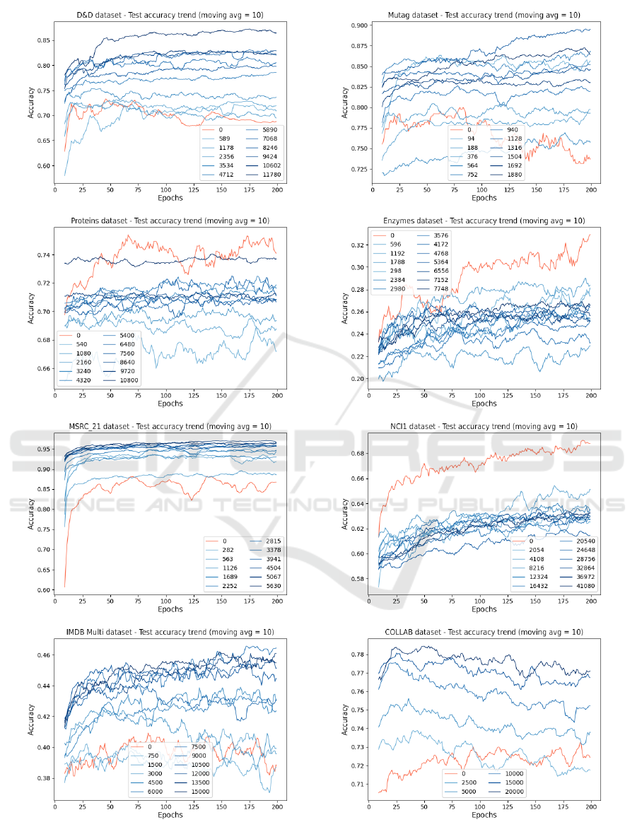
Figure 2: Accuracy results of the test set for the datasets’ graph classification training with 5 cluster division. For clarity it is

shown the moving average of the results with W = 10. The red curve is the untouched dataset training, the other curves are the

augmented runs, where the darker the color the bigger is the augmentation. In the legend are reported the number of graphs

GAMS decreases the performance with respect to the

original training set, confirming the hypothesis that

in these datasets the structure is not as important for

classification.

tracting and swapping these substructures from train-

ing graph with the same label. This provides an aug-

mentation approach that is data-driven, in the sense

that the swapped-in motifs are directly observed from

the dataset, but that not require to be learned nor it

is in any way coupled with the learning algorithm

adopted for the final classification problem.

proach is capable of providing very substantive in-

creases in performance for datasets where the struc-

Bertsekas, D. P. (1992). Auction algorithms for network

Chen, D., Lin, Y., Li, W., Li, P., Zhou, J., and Sun, X.

Gilmer, J., Schoenholz, S. S., Riley, P. F., Vinyals, O., and

Rong, Y., Huang, W., Xu, T., and Huang, J. (2019). Drope-

Shi, J. and Malik, J. (2000). Normalized cuts and image

Weisfeiler, B. and Lehman, A. A. (1968). A reduction of

Zhao, T., Liu, Y., Neves, L., Woodford, O., Jiang, M., and