Relative Position φ-Descriptor Computation for Complex Polygonal

Objects

Tyler Laforet and Pascal Matsakis

School of Computer Science, University of Guelph, Stone Rd E, Guelph, Canada

Keywords:

Image Descriptors, Relative Position Descriptors, φ-Descriptor, Spatial Relationships, Vector Objects,

2-Dimensional.

Abstract:

In regular conversation, one often refers to the spatial relationships between objects via their positions relative

to each other. Relative Position Descriptors (RPDs) are a type of image descriptor tuned to extract these spatial

relationships from pairs of objects. Of the existing RPDs, the φ-descriptor covers the widest variety of spatial

relationships. Currently, algorithms exist for its computation in the case of both 2D raster and vector objects.

However, the algorithm for 2D vector calculation can only handle pairs of simple polygons and lacks some

key features, including support for objects with disjoint parts/holes, shared polygon vertices/edges, and various

spatial relationships. This paper presents an approach for complex polygonal object φ-descriptor computation,

built upon the previous. The new algorithm utilizes the analysis of object boundaries, polygon edges that

represent changes in spatial relationships, and brings it more in-line with the 2D raster approach.

1 INTRODUCTION

In regular conversation, one often refers to the loca-

tions of objects, people, and places using their posi-

tion in relation to others. These relative positions are

usually described through various prepositions, which

are divided into three major groups: directional (e.g.,

in front of, above), topological (e.g., inside, apart),

and distance (e.g., nearby, far away). To analyze

these relative positions, relative position descriptors

(RPDs) can be utilized. A type of image descriptor,

these RPDs extract the spatial relationships held be-

tween two objects in an image, reporting them quanti-

tatively. Of the existing RPDs, the φ-descriptor (Mat-

sakis et al., 2015) is the ﬁrst capable of modeling all

three types of spatial relationships. Currently, meth-

ods exist for its derivation in the case of 2D raster

(pixel-based) (Naeem, 2016) and vector (polygonal)

(Kemp, 2019; Kemp et al., 2020) objects. How-

ever, the 2D vector approach lacks the ability to prop-

erly support the surrounds relationship, disjoint ob-

ject parts, holes, and shared polygon vertices/edges.

The aim of this work is to show that these lim-

itations can be removed by bringing the design of

the vector approach closer to the raster approach. To

this end, a redesign of the vector approach is intro-

duced. The revised approach is based on the analy-

sis of object boundaries, polygon edges that represent

changes in spatial relationships. Through this revision

the complex polygon objects and spatial relationships

that previously lacked support can be handled.

2 BACKGROUND

Here, we provide an overview of relative position de-

scription (Section 2.1) and the φ-descriptor (Section

2.2).

2.1 Relative Position Description

Relative position descriptors (RPDs) are a type of im-

age descriptor made to extract the position of two ob-

jects in relation to each other. These relative positions

are described using prepositions, which, as stated

previously, are divided into directional, topological

and distance spatial relationships. RPDs provide a

quantitative description of these spatial relationships,

and form the basis of qualitative descriptions (Francis

et al., 2018). As these relative positions are an impor-

tant part of everyday speech, RPDs have found use in

a variety of ﬁelds, including human-robot interaction

(Skubic et al., 2004), medical imaging (Colliot et al.,

2006), mineﬁeld risk estimation (Chan et al., 2005),

symbol recognition (Santosh et al., 2012) and robot

264

Laforet, T. and Matsakis, P.

Relative Position -Descriptor Computation for Complex Polygonal Objects.

DOI: 10.5220/0010823400003122

In Proceedings of the 11th International Conference on Pattern Recognition Applications and Methods (ICPRAM 2022), pages 264-271

ISBN: 978-989-758-549-4; ISSN: 2184-4313

navigation (Skubic et al., 2001).

Relative position description through the identiﬁ-

cation of spatial relationships was ﬁrst suggested in

(Freeman, 1975), and was later reﬁned into the use

of RPDs (Miyajima and Ralescu, 1994). Many RPD

models have since been developed, including the an-

gle histogram (Miyajima and Ralescu, 1994), force

histogram (Matsakis and Wendling, 1999), Allen

histograms (Allen, 1983), R-histogram (Wang and

Makedon, 2003), R*-histogram (Wang et al., 2004),

spread histogram (Kwasnicka and Paradowski, 2005),

and visual area histogram (Zhang et al., 2010). Of the

existing models, few have support for vector (polygo-

nal) objects, and most focus only on one type of spa-

tial relationship (Naeem and Matsakis, 2015).

2.2 φ-Descriptor

The φ-descriptor, introduced in (Matsakis et al.,

2015), is the ﬁrst RPD capable of mapping all three

types of spatial relationships, including the surrounds

relationship previously only targeted by the spread

histogram. As such, the φ-descriptor covers a wider

breadth of spatial relationships than its contempo-

raries, and serves as their successor. Here, we cover

the basic concepts forming the φ-descriptor (Section

2.2.1) and the existing algorithms for its computation

(Section 2.2.2).

2.2.1 Basic Concepts

The φ-descriptor is a set of histograms denoting rela-

tive position information in an image, derived from

a set of elementary (low-level) spatial relationships

(Allen, 1983). Similar low-level relationships can

be grouped to form medium-level relationships (φ-

groups). As shown in Figure 1, φ-groups are derived

by taking linear slices of the objects and matching

them to low-level relationships via analysis of object

membership changes (object entries/exits). Many of

these relationships correspond to pairs of object en-

tries/exits (point-pairs), with similar sets forming into

ten distinct φ-groups. The width φ-group, then, is the

total area covered by these point-pair-based φ-groups

(region of interaction). Additionally, the encloses and

divides φ-groups represent instances of one object lo-

cated between segments of the other. Each of these

φ-groups correspond to histogram values, represent-

ing their total area and height for each direction in

a direction set (as shown in Table 1); as the number

of directions increases, so too does the completeness

of the extracted information. These values can then

be further analyzed to derive high-level relationships

(Francis et al., 2018), such as the surrounds relation-

ship.

Table 1: Part of a φ-descriptor for an example pair of ob-

jects. (Kemp, 2019; Kemp et al., 2020).

φ-Group

0 5 ...

RoI area 310009 311138 ...

Roi length 516.681 533.891 ...

Void area 404 234 ...

Void length 202 36.137 ...

Arg area 7769 7819 ...

Arg length 75.062 70.710 ...

Ref area 7863 9200 ...

Ref length 129.966 120.720 ...

... ... ... ...

Figure 1: The point-pair-based φ-groups, and the encloses,

divides, and width φ-groups. Dark-grey represents object

A. Light-grey represents object B. Note that the region in

the middle of the point-pair-based φ-groups (|pq|) is to be

assigned the φ-group. (Matsakis et al., 2015).

2.2.2 Existing φ-Description Algorithms

Currently, there are two main methods for calculating

the φ-descriptor. The ﬁrst obtains linear slices of a

2D raster image by passing through lines (rays) and

analyzing corresponding groups of sequential pixels

to determine the object entries/exits and their corre-

sponding φ-groups (Naeem, 2016). The second, de-

signed for 2D vector images, operates by determin-

ing polygon vertices (polynodes) where φ-groups are

known to change (points of interest) and similarly

passing rays through them (Kemp, 2019; Kemp et al.,

2020). Point-pairs are then determined by analyzing

the changes in object membership at each polynode

on the ray, with areas representing these φ-groups (φ-

regions) extracted by traversing edges of the polygon

objects counter-clockwise from each polynodes.

Unfortunately, the current 2D-vector-based ap-

proach suffers from several drawbacks. Firstly, the al-

gorithm assumes that each ray polynode cleanly maps

to the φ-regions above them, and thus uses them as

Relative Position -Descriptor Computation for Complex Polygonal Objects

265

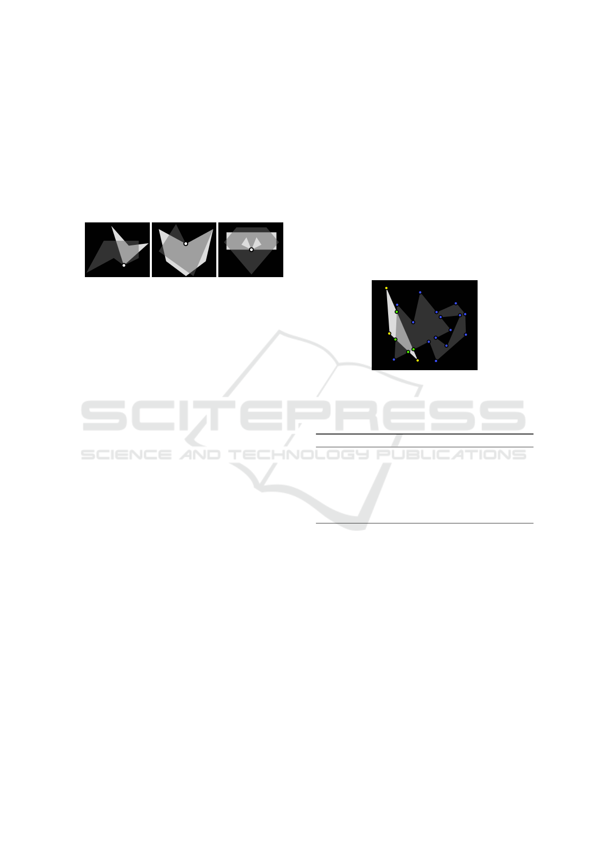
the point-pairs. However, a single polynode can map

to countless φ-regions, as demonstrated in Figure 2.

The algorithm only supports this scenario up to two

φ-regions, hindering its ability to support objects with

disjoint parts, holes or shared polygon vertices/edges.

This also hinders its ability to properly detect the fol-

lows, leads, and starts φ-groups. Additionally, the ap-

proach has no support for the encloses and divides φ-

groups. As a result, the current method falls short of

the goals of a φ-descriptor algorithm.

Figure 2: Example pairs of objects unsupported by the cur-

rent 2D vector φ-descriptor algorithm. Each of these fea-

ture polynodes that map to more than two φ-regions directly

above them. The relevant polynodes have been marked.

3 BOUNDARY-BASED 2D

VECTOR φ-DESCRIPTION

Here, we provide an overview of the revised algo-

rithm for 2D-vector φ-description; it has been de-

signed with the goals of removing the existing lim-

itations and simplifying the approach through the

use of polygon edges representing object entries/exits

(boundaries). Included in this overview are the pre-

processing steps (Section 3.1), points of interest and

rays (Section 3.2), boundaries (Section 3.3), φ-regions

(Section 3.4), φ-group ﬁne-tuning (Section 3.5) and

φ-descriptor output (Section 3.6).

3.1 Preprocessing

To begin, the pair of objects of the 2D vector im-

age are inputted into the program as sets of simple

polygons. Each polygon is made up of a doubly-

linked list of polygon vertices (polynodes), each con-

taining an x/y coordinates variable shared amongst

all other shared/overlapping polynodes. To ensure

compatibility with later steps of the process, a poly-

gon clipping algorithm (Margalit and Knott, 1989)

(Kim and Kim, 2006) (Wilson, 2013) is applied to

union/subtract polygons for removal of unnecessary

edges. Next, a sweep-line intersection detection algo-

rithm (Zalik, 2000) is utilized to ﬁnd overlapping co-

ordinates in the edges of pairs of object polygons, in-

serting new vertices as necessary (as shown in Figure

3). Finally, the object membership (source) of each

polynode is recorded, to be used in analysis of object

entries/exits; they can be assigned with either an ob-

ject source of A (belongs to object A), B (belongs to

object B) or I (belongs to both objects). Object source

N (belongs to neither object) is also deﬁned, though

no polynode can be set with this.

As mentioned in Section 2.2.1, a direction set is

utilized for calculation of the φ-descriptor. To sim-

plify the process of determining the φ-regions of each

direction, the objects are to be rotated, in a pro-

cess summarized in Algorithm 1 (Kemp, 2019; Kemp

et al., 2020), so all directions may be analyzed left-to-

right. As discussed later, optimizations are possible

by analyzing both direction θ and the direction oppo-

site (−θ = θ + 180

◦

) simultaneously; as such, an even

number of evenly-spaced directions are to be utilized.

Figure 3: An example pair of objects with object sources

set for their polynodes. Blue dots represent polynodes with

object source A (dark-grey). Yellow dots represent polyn-

odes with object source B (light-grey). Green dots represent

polynodes with object source I (both objects).

Algorithm 1: Object Rotation (Kemp et al., 2020).

1: centroid = mean of all vertex coordinates in Ob-

jects A or B

2: for all Coordinate c in Objects A or B do

3: ∆C = c - centroid

4: c.x = centroid.x + ∆C.x * cosθ - ∆C.y * sinθ

5: c.y = centroid.y + ∆C.x * sinθ - ∆C.y * cosθ

3.2 Points of Interest and Rays

As discussed in Section 2.2.2, both previous ap-

proaches pass rays through the image to segment

the objects into linear slices for φ-group derivation;

for the 2D vector speciﬁcally, these rays are passed

through the polynodes with the space between form-

ing the linear slices. The naive approach, then, is

to pass rays through every polynode of the object

pair; however, many polynodes do not contribute any

changes to φ-groups, as object entries/exits do not

change above/below them (see Figure 4). As such,

it is necessary to identify polynodes that do cause

such changes in object membership (points of inter-

est). As shown in Figure 5, the polynodes identiﬁed

as points of interest are as follows: object edge inter-

sections, local minima and maxima, bounding polyn-

ICPRAM 2022 - 11th International Conference on Pattern Recognition Applications and Methods

266

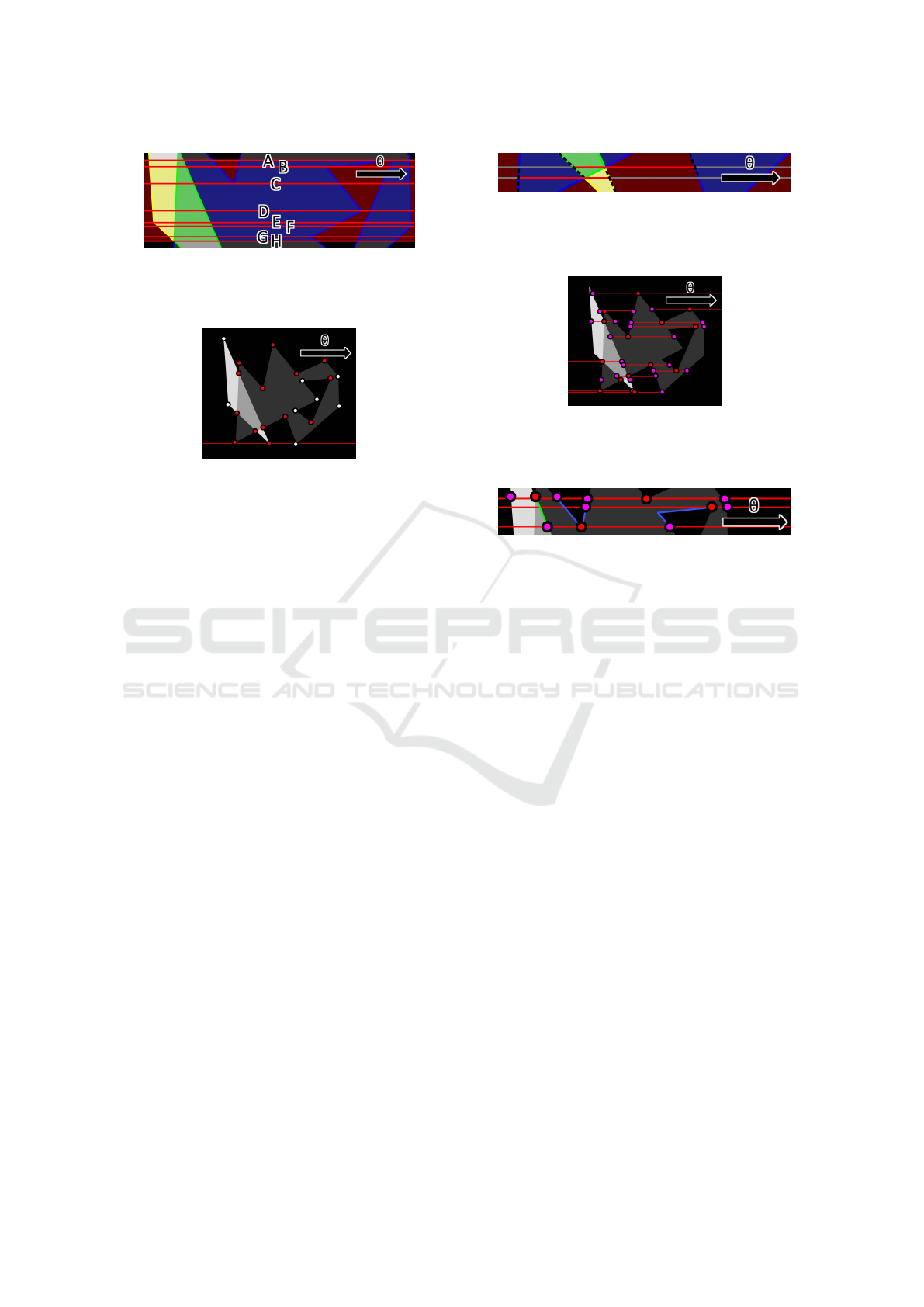
Figure 4: A subset of rays passed through all polynodes of a

pair of objects in direction θ. Note that between rays A and

C, the polygon edges correspond to the same set of object

entries/exits. Similar applies between rays C and H.

Figure 5: The points of interest for an example pair of ob-

jects in direction θ. Points of interest are marked with red

dots. Red lines represent the bounding rays of the region of

interaction. Note that only polynodes within the region of

interaction are considered.

odes of the region of interaction, and neighbouring

polynodes horizontal to these other points of interest

(Kemp, 2019; Kemp et al., 2020).

Horizontal rays are then passed through the ob-

ject pair at each point of interest; intersections with

polygon edges (ray endpoints) are stored, inserting

new polynodes if necessary. Again, it is noted that

only certain polynodes have changes in object mem-

bership above/below them. As such, to construct the

minimal amount of point-pair-based φ-regions, only

such polynodes are considered. As shown in Figure 6,

these are the points of interest and their neighbouring

ray endpoints, which are marked as φ-group-dividing

polynodes. Figure 7 demonstrates the result of these

steps applied to an example pair of objects.

3.3 Boundaries

As discussed in Section 2.2.2, limitations with the

original 2D vector algorithm stemmed from the use of

ray endpoints as point-pairs, as a single endpoint can

map to countless object entries/exits, and by extension

φ-regions. To remove these limitations, we introduce

the concept of object boundaries, polygon edges be-

tween rays that directly represent entries/exits within

the linear slice. By analyzing these boundaries, we

calculate φ-groups and their corresponding φ-regions

exactly as was done in the raster approach. From

each dividing polynode on a ray, we scan every neigh-

bouring edge above until another dividing polynode

is found. Note that multiple rays may be crossed

Figure 6: Rays from an example set of objects. Note that

the grey ray segments represent the same object entries/exits

above/below them at their endpoints (shown with dotted

lines), and thus, do not represent a change in φ-groups.

Figure 7: Dividing polynodes for an example pair of ob-

jects. Red dots represent points of interest. Purple dots rep-

resent other dividing polynodes. Ray segments deﬁned by

points of interest are included between dividing polynodes.

Figure 8: Boundaries extracted from a ray (bottom-most)

for an example pair of objects. Blue boundaries belong to

object A. Green boundaries belong to both objects. Note

that the two leftmost boundaries cross multiple rays due to

not encountering a dividing polynode along those rays.

where no dividing polynodes are found, to facilitate

extraction of minimal point-pair-based φ-regions (see

Figure 8); by deﬁnition, only a single path will be

traversable until the next dividing polynode is found.

Also note that rays are ignored if their linear slice di-

rectly above has participation of one or less objects, as

it does not contribute to the relative position of the ob-

jects; all boundaries end at the ray, even if no dividing

polynode would be found, and all polynodes of the

next, non-ignored ray are treated as dividing polyn-

odes. The encountered polynodes are then stored as

a boundary, with its object source dependent on the

aggregate of the object sources of its polynodes (I if

both objects participate, A or B otherwise).

3.4 φ-Regions

As stated in Section 3.3, φ-regions are determined

by scanning the object boundaries for object en-

tries/exits, analyzing them to determine φ-groups us-

ing methods similar to the 2D raster approach. For

each ray, we scan across the set of object boundaries

who lay above the ray, left-to-right. For each pair

of sequential boundaries, whose starting endpoint is

the current ray (for minimal φ-regions), we analyze

the object entries/exits they represent to determine the

point-pair-based φ-groups for both directions θ and

Relative Position -Descriptor Computation for Complex Polygonal Objects

267

Figure 9: Extension of boundaries (blue lines) across rays

to form a φ-region from an example pair of objects.

Figure 10: Point-pair-based φ-regions for an example pair

of objects in direction θ. Blue regions belong to object A.

Yellow regions belong to object B. Green regions belong to

both objects. Red regions belong to neither object.

Figure 11: The point-pair-based φ-groups of the φ-regions

in Figure 10, in direction θ (left) and direction −θ (right).

−θ. Then, as shown in Figure 9, we extend the bound-

aries from their ending endpoints until both lay on the

same ray (both are dividing polynodes). The φ-region

for the corresponding φ-groups, then, is found by in-

serting polygon edges between the starting/extended-

ending endpoints of the two boundaries. The results

of this process are shown in Figures 10 and 11.

Similar methods are used to extract φ-regions for

the encloses and divides φ-groups. For each ray,

we scan across the set of object boundaries between

the current and above rays, left-to-right. For ev-

ery entry-exit pair from object A/B (not I), we con-

nect the two boundaries with polygon edges along the

current/above rays and store them as a potential di-

vides/encloses φ-region for directions θ and −θ. If,

then, an entry to the opposite object B/A is found, we

check if an exit to the object existed previously. If so,

all potential divides/encloses φ-regions are stored for

later use; otherwise, they are tossed. The results of

this process are shown in Figure 12. Note that this

method does not ﬁnd minimal encloses and divides

φ-regions, which is left as future work.

Figure 12: Encloses and divides φ-regions for an example

pair of objects in direction θ. Blue regions depict the divides

φ-group. Yellow regions depict the encloses φ-group.

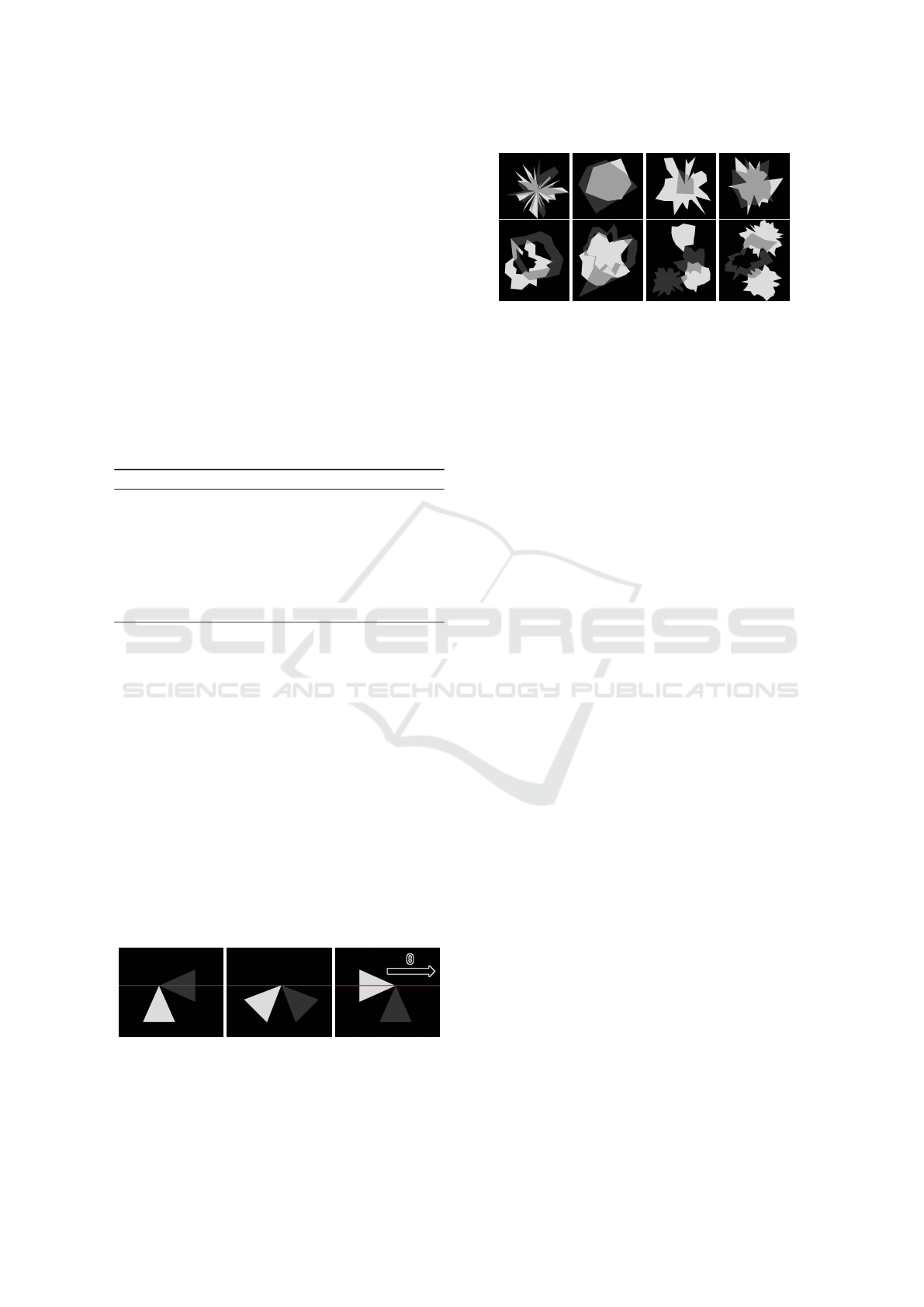
Figure 13: Examples of object pairs that touch but have no

follows, leads or starts φ-groups under the approach in Sec-

tion 3.4. Note that the objects touch at a shared polynode;

as such, the behaviour goes undetected as the corresponding

leads (left) and starts (right) relationships are not found in

the φ-regions above or below the ray (shown in red).

3.5 Fine-tuning

While the steps outlined so far cover the most sce-

narios, object pairs with missing φ-group detections

remain. Particularly, cases where two objects touch at

a single vertex, such as those in Figure 13, should ex-

hibit follows, leads, or starts φ-groups. However, as

they touch at an inﬁnitesimally-small 1D area, these

φ-groups go unreported. As such, we include ﬁne-

tuning methods to properly represent these relation-

ships (Francis et al., 2021). For each ray, we scan

its endpoints left-to-right, tracking how object source

changes along the ray; note that this depends on the

aggregate of object entries/exits above and below the

ray (e.g., A above and B below equals I along the ray).

Φ-groups are then determined in the point-pair-based

method; if follows, leads or starts is detected in direc-

tion θ (or −θ), then they are marked as ﬁne-tuned.

A special case remains when objects touch such

that no rays pass through segments of both (see Fig-

ure 14). To handle these, check if a polynode is a sin-

gle object minima/maxima. If so, check if the source

of their ray segments change from A/B to N, such that

the endpoint is an object B/A extrema; if so, set fol-

lows/leads as ﬁne-tuned for direction θ; direction −θ

is set if the opposite change occurs (N to A/B).

3.6 Descriptor Output

Once φ-regions have been calculated for direction θ,

all φ-regions of the same φ-group have their areas

ICPRAM 2022 - 11th International Conference on Pattern Recognition Applications and Methods

268

(see Algorithm 2) and heights (difference in y-value

of their top and bottom-most vertices) summed and

stored in the descriptor (as shown in Section 2.2.1). If

follows, leads or starts are ﬁne-tuned and would have

zero area/height otherwise, they’re recorded as “0+”.

Note that the width φ-group consists of all point-pair-

based φ-regions; height is the difference in y-value of

the top and bottom-most rays, with height above ig-

nored rays (as mentioned in Section 3.3) subtracted.

As mentioned in Section 2.2.1, the same φ-regions

are found in directions θ and −θ, and thus are cal-

culated simultaneously. It should be noted, however,

that the point-pair-based φ-regions may correspond to

different φ-groups in the opposite direction (as shown

in Figure 11); for φ-regions with the same point-pair-

based φ-groups in both directions, their areas and

heights are halved (Matsakis et al., 2015).

Algorithm 2: φ-Region Area (Kemp et al., 2020).

1: area = 0.0

2: j = number of PolyNodes in phiRegion - 1

3: for i = 0, number of PolyNodes in phiRegion do

4: area += (phiRegion[j].x + phiRegion[i].x) *

(phiRegion[j].y - phiRegion[i].y)

5: j = i

6: area = abs(area)

4 EXPERIMENTS

Here, we detail the experiments used to validate

the performance of the boundary-based 2D vector

φ-description algorithm, including the methodology

(Section 4.1) and the results (Section 4.2).

4.1 Methodology

To evaluate the performance of the revised 2D vector

φ-description algorithm, automated tests were used.

To begin, polygon object pairs are randomly gener-

ated using an approach previously used for testing

φ-descriptor algorithms (Kemp, 2019; Kemp et al.,

2020). Such objects tend to exhibit a spiky pattern

Figure 14: An example pair of objects that touch, shown

at multiple rotations. Note that there is not a φ-region that

corresponds to the follows or starts behaviour above or be-

low the given ray (shown in red), nor is there a rotation that

leads to 1D segments of both objects lying on the ray.

Figure 15: Examples of simple (top) and complex (bottom)

polygon objects generated for testing against the 2D raster

and revised vector φ-description algorithms.

(see Figure 15), and by extension a wide range of spa-

tial relationships. For testing against the previous vec-

tor algorithm, 250 single polygon objects were gener-

ated this way. Additionally, a modiﬁed approach was

used to generate 250 complex object pairs, covering

cases unsupported by the previous vector algorithm

(see Section 2.2.2). A random number of polygons

are selected, with the ﬁrst two having sources A and B

respectively; the center of each polygon is randomly

offset from the previous. After generating each poly-

gon, a smaller copy may be added as a hole. Poly-

gons may also inherit a vertex/edge from the previ-

ous. These changes ensure the presence of previously

unsupported scenarios within the test set, as shown in

Figure 15. For testing with the 2D raster approach,

each object pair is rasterized at varying resolutions.

For each object pair, φ-descriptors are generated

for the 2D raster and revised vector algorithms (and

original vector if supported); output is normalized

by dividing each φ-group’s area/height by that of the

width φ-group, to ensure independence from factors

like image resolution. Two similarity measures are

used to compare the normalized descriptors, as done

previously (Naeem, 2016) (Kemp, 2019; Kemp et al.,

2020). The ﬁrst, MinMax, is the sum of minimum

values of each shared datapoint divided by the sum of

maximums. The second, SubAdd, takes the sum of

differences of each shared datapoint, divides it by the

sum of sums, and subtracts it from 1.00. The closer

these similarity values are to 1.00, the more similar

the descriptors are (Kemp, 2019; Kemp et al., 2020).

4.2 Results

As stated previously, 500 object pairs were gener-

ated and tested against the three algorithms (ignoring

the original vector when unsupported). As shown in

Figure 16, the revised vector approach displays high

similarity with the raster approach; results averaged

above 90% in all measures for images with resolu-

tion greater than 100x100. It was also observed that

similarity increased as raster image resolution did, as

Relative Position -Descriptor Computation for Complex Polygonal Objects

269

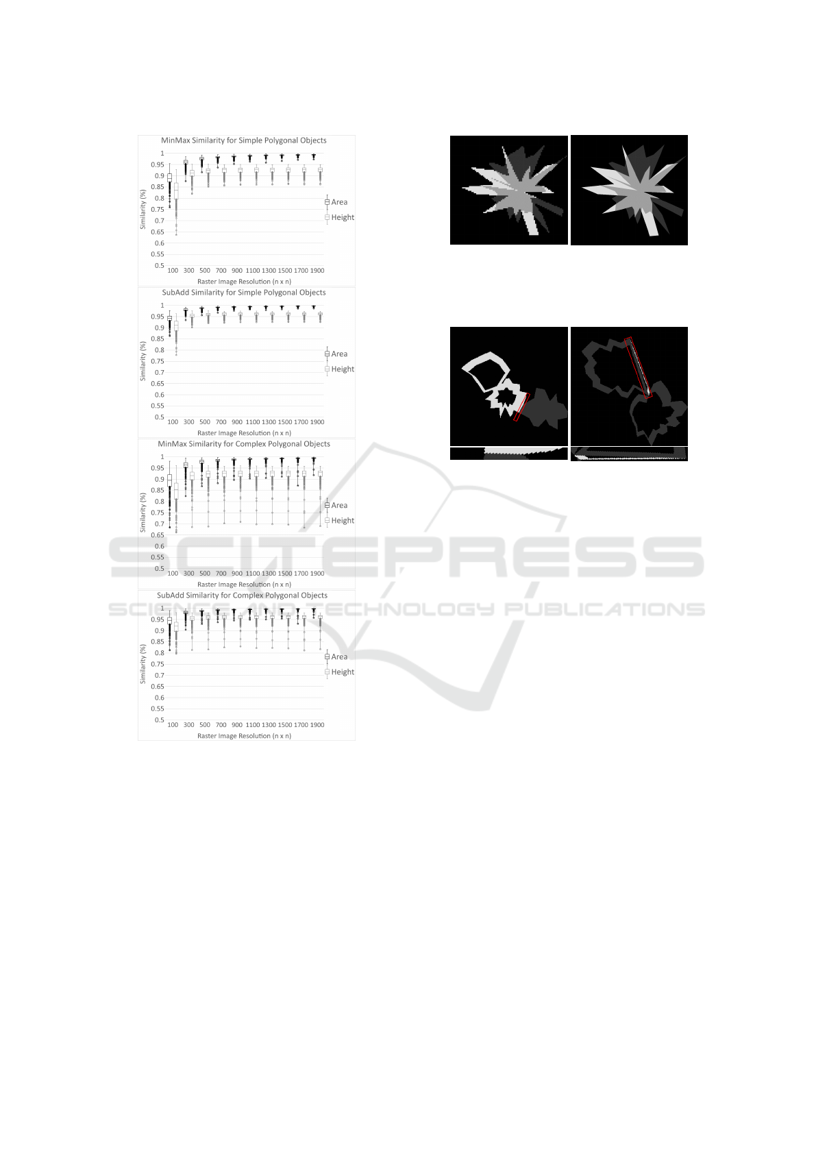
Figure 16: MinMax and SubAdd similarity between the out-

puts of the 2D raster and revised vector φ-description algo-

rithms for the simple and complex polygon object dataset.

information becomes more complete (see Figure 17).

Generally lower height similarities were noted for

similar reasons; as shown in Figure 18, affected object

pairs contain rasterized edges that, when rotated to

nearly horizontal, become jagged. Consequentially,

repeated object entries/exits and generation of large

amounts of φ-regions occur, resulting in heights much

larger than the vector approach, due to it calculation

as the sum of the heights of corresponding φ-regions.

It is noted, however, that output is correct for both

algorithms. Additionally, it was found that the new

and old vector algorithms produced identical output,

Figure 17: An object pair that displayed low similarity

scores at raster image resolution 100x100. Thin edges were

rasterized such that they appear to be made of distinct parts,

and nearly parallel edges located close to each other were

rasterized such that they appear to be shared.

Figure 18: Two of the worst complex object pairs for height

similarity, shown at 300x300 resolution. Both contain an

edge that, when nearly horizontal, causes many object en-

tries/exits. Each is shown in the offending direction.

excluding φ-groups originally unsupported. Overall,

these results show that the newly supported scenarios

do not have a negative impact on output similarity.

Figure 19 displays the runtime results for the 2D

raster, original vector and revised vector algorithms.

Generally, as the number of polynodes increases, run-

time needed increases faster for the vector than the

raster. The performance of both vector approaches

depends directly on the complexity of the inputted ob-

jects in regard to the number of polynodes, or specif-

ically the points of interest. In contrast, the perfor-

mance of the raster approach depends mostly on the

resolution of the inputted image, growing more lin-

early in regard to the number of polynodes. Ulti-

mately, the new approach to 2D vector φ-description

outperforms that of the original vector, and maintains

comparable performance to that of the raster.

5 CONCLUSIONS

In this paper, we have introduced a revised approach

to 2D vector φ-descriptor calculation. By mapping the

concept of object edges (boundaries) to that of object

entries/exits, many limitations seen with the previous

approach have been eliminated. The performance of

this new algorithm was validated using 500 polygon

object pairs, covering a wide range of objects previ-

ICPRAM 2022 - 11th International Conference on Pattern Recognition Applications and Methods

270

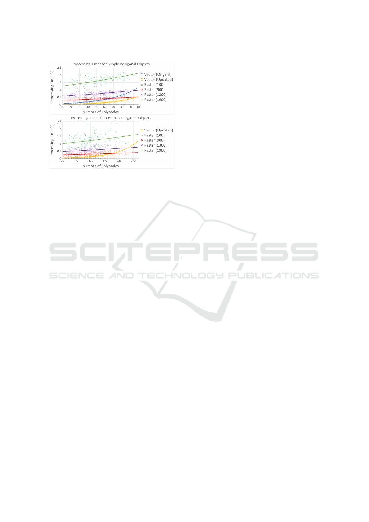
Figure 19: Processing times for the 2D raster, original vec-

tor, and revised vector φ-description algorithms for the sim-

ple and complex polygon object datasets.

ously and newly supported. Overall, the results show

that the new algorithm outperforms the previous vec-

tor approach whilst still maintaining high descriptor

similarity and comparable runtime performance to the

raster. Ultimately, the new boundary-based 2D vector

φ-description algorithm has been shown to be a capa-

ble successor to its predecessor, simplifying and im-

proving upon it. Applications of this work are those

with the need to detect a wide variety of spatial re-

lationships from 2D vector information (e.g., geo-

graphic information systems, human-robot communi-

cation, medical imaging, etc.). Future work includes

runtime performance improvements, such as the cre-

ation of minimal encloses and divides φ-regions.

REFERENCES

Allen, J. F. (1983). Maintaining knowledge about temporal

intervals. Commun. ACM, 26:832–843.

Chan, J., Sahli, H., and Wang, Y. (2005). Semantic risk es-

timation of suspected mineﬁelds based on spatial re-

lationships analysis of mineﬁeld indictors from multi-

level remote sensing imagery. Proceedings of SPIE -

The International Society for Optical Engineering.

Colliot, O., Camara, O., and Bloch, I. (2006). Integra-

tion of fuzzy spatial relations in deformable mod-

els—application to brain mri segmentation. Pattern

Recognition, 39:1401–1414.

Francis, J., Laforet, T., and Matsakis, P. (2021). Models

of spatial relationships based on the φ-descriptor. In

preparation.

Francis, J., Rahbarnia, F., and Matsakis, P. (2018). Fuzzy

nlg system for extensive verbal description of relative

positions. In 2018 IEEE International Conference on

Fuzzy Systems (FUZZ-IEEE), pages 1–8.

Freeman, J. (1975). The modelling of spatial relations.

Computer Graphics and Image Processing, 4(2):156–

171.

Kemp, J. (2019). Contributions to relative position descrip-

tor computation in the case of vector objects.

Kemp, J., Laforet, T., and Matsakis, P. (2020). Computation

of the φ-descriptor in the case of 2d vector objects. In

ICPRAM, pages 60–68.

Kim, D. H. and Kim, M.-J. (2006). An extension of polygon

clipping to resolve degenerate cases. Computer-aided

Design and Applications, 3:447–456.

Kwasnicka, H. and Paradowski, M. (2005). Spread his-

togram - a method for calculating spatial relations be-

tween objects. In CORES.

Margalit, A. and Knott, G. (1989). An algorithm for com-

puting the union, intersection or difference of two

polygons. Computers & Graphics, 13:167–183.

Matsakis, P., Naeem, M., and Rahbarnia, F. (2015). In-

troducing the φ-descriptor - a most versatile relative

position descriptor. In ICPRAM.

Matsakis, P. and Wendling, L. (1999). A new way to repre-

sent the relative position between areal objects. IEEE

Transactions on Pattern Analysis and Machine Intel-

ligence, 21(7):634–643.

Miyajima, K. and Ralescu, A. (1994). Spatial organization

in 2d segmented images: Representation and recogni-

tion of primitive spatial relations. Fuzzy Sets and Sys-

tems, 65(2):225–236. Fuzzy Methods for Computer

Vision and Pattern Recognition.

Naeem, M. (2016). A most versatile relative position de-

scriptor.

Naeem, M. and Matsakis, P. (2015). Relative position de-

scriptors - a review. In ICPRAM.

Santosh, K., Lamiroy, B., and Wendling, L. (2012). Symbol

recognition using spatial relations. Pattern Recogni-

tion Letters, 33:331–341.

Skubic, M., Chronis, G., Matsakis, P., and Keller, J. (2001).

Spatial relations for tactical robot navigation. In SPIE

Defense + Commercial Sensing.

Skubic, M., Perzanowski, D., Blisard, S., Schultz, A.,

Adams, W., Bugajska, M., and Brock, D. (2004). Spa-

tial language for human-robot dialogs. IEEE Transac-

tions on Systems, Man, and Cybernetics, Part C (Ap-

plications and Reviews), 34(2):154–167.

Wang, Y. and Makedon, F. (2003). R-histogram: Quanti-

tative representation of spatial relations for similarity-

based image retrieval. pages 323–326.

Wang, Y., Makedon, F., and Chakrabarti, A. (2004). R*-

histograms: Efﬁcient representation of spatial rela-

tions between objects of arbitrary topology. pages

356–359.

Wilson, J. (2013). Polygon Subtraction in 2 or 3 Dimen-

sions.

Zalik, B. (2000). Two efﬁcient algorithms for determining

intersection points between simple polygons. Com-

puters & Geosciences, 26:137–151.

Zhang, K., Wang, K.-p., Wang, X.-j., and Zhong, Y.-x.

(2010). Spatial relations modeling based on visual

area histogram. In 2010 11th ACIS International Con-

ference on Software Engineering, Artiﬁcial Intelli-

gence, Networking and Parallel/Distributed Comput-

ing, pages 97–101.

Relative Position -Descriptor Computation for Complex Polygonal Objects

271