
Caterpillar Inclusion: Inclusion Problem for Rooted Labeled Caterpillars
Tomoya Miyazaki, Manami Hagihara and Kouich Hirata
Kyushu Institute of Technology, Kawazu 680-4, Iizuka 820-8502, Japan
Keywords:
Caterpillar Inclusion, Tree Inclusion, Rooted Labeled Caterpillar, Rooted Labeled Unordered Tree.
Abstract:
In this paper, we investigate an inclusion problem for rooted labeled caterpillars (resp., caterpillars, for short),
which we call a caterpillar inclusion. The caterpillar inclusion is to determine whether or not a text caterpillar
T achieves to a pattern caterpillar P by deleting vertices in T. Then, we design the algorithm of the caterpillar
inclusion for P and T in O((h + H)σ) time, where h is the height of P, H is the height of T and σ is the
number of labels occurring in P and T. Also we give experimental results for the algorithm by using real data
for caterpillars.
1 INTRODUCTION
The pattern matching for tree-structured data such
as HTML and XML documents for web mining or
DNA and glycan data for bioinformatics is one of the
fundamental tasks for information retrieval or query
processing. As such pattern matching for rooted la-
beled unordered trees, an unordered tree inclusion (an
inclusion, for short) is the problem of determining
whether or not an unordered tree P called a pattern
tree is included in an unordered tree T called a text
tree, that is, T achieves to P by deleting vertices in
T. However, the inclusion is known to be intractable,
that is, NP-complete (Kilpel¨ainen and Mannila, 1995;
Matou˘sek and Thomas, 1992).
In order to overcome such intractability, several
researches have developed the tractable variations of
the inclusion such as a top-down inclusion (Shamir
and Tsur, 1999), a bottom-up inclusion (Valiente,
2002), an LCA-preserving inclusion (Valiente, 2005)
1
and an isolated-subtree inclusion (Hokazono et al.,
2012). The first three variations are formulated by
restricting the scope of the deletion of vertices to
just leaves, just roots and just either leaves or ver-
tices with one child, respectively. Also the top-down
(resp., bottom-up) inclusion coincides with the top-
down (resp., bottom-up) unordered subtree isomor-
phism (cf., (Valiente, 2002)). On the other hand, the
1
While Valiente (Valiente, 2005) has called it a con-
strained inclusion, the definition of (Valiente, 2005) is cor-
responding to an LCA-preserving distance or a degree-2
distance (Zhang et al., 1996). Hence, we call it an LCA-
preserving inclusion.
several algorithms to compute unordered tree inclu-
sion have been designed as the exact exponential al-
gorithms (Akutsu et al., 2021; Kilpel¨ainen and Man-
nila, 1995).
Note that the proof of NP-completeness for the
inclusion implies the structural restriction of the
tractability for the inclusion that the height of a text
tree is at most 2 or the degree of a text tree is bounded
by some constant (Kilpel¨ainen and Mannila, 1995;
Matou˘sek and Thomas, 1992). In this paper, we give
another structural restriction providing the limitation
of the tractability for the inclusion as a rooted la-
beled caterpillar (a caterpillar, for short) (cf., (Gal-
lian, 2007)). The caterpillar is an unordered tree
transformed to a rooted path after removing all the
leaves in it.
The caterpillar provides the structural restriction
of the tractability of computing the edit distance for
unordered trees (Muraka et al., 2018). It is known
that the problem of computing the edit distance be-
tween unordered trees is MAX SNP-hard (Zhang and
Jiang, 1994). This statement also holds even if two
trees are binary, the maximum height is at most 3
or the cost function is the unit cost function (Akutsu
et al., 2013; Hirata et al., 2011). On the other hand,
we can compute the edit distance between caterpil-
lars in O(h
2
λ
3
) time in the general cost function and
O(h
2
λ) time under the unit cost function, where h is
the maximum height of the two caterpillars and λ is
the maximum number of leaves in the two caterpil-
lars (Muraka et al., 2018)
2
.
2
This time complexity is different from the result in
(Muraka et al., 2018), because it contains some errors. See
280
Miyazaki, T., Hagihara, M. and Hirata, K.
Caterpillar Inclusion: Inclusion Problem for Rooted Labeled Caterpillars.
DOI: 10.5220/0010826300003122
In Proceedings of the 11th International Conference on Pattern Recognition Applications and Methods (ICPRAM 2022), pages 280-287
ISBN: 978-989-758-549-4; ISSN: 2184-4313
Copyright
c
2022 by SCITEPRESS – Science and Technology Publications, Lda. All rights reserved
Hence, in this paper, we investigate a caterpil-
lar inclusion of determining whether or not a pat-
tern caterpillar P is included in a text caterpillar T.
Then, we design the algorithm CATINC of determin-
ing whether or not P is included in T in O((h+ H)σ)
time, where h is the height of P, H is the height of T
and σ is the number of labels occurring in P and T.
Also, we give experimental results for the algorithm
CATINC by using real caterpillar data.
2 PRELIMINARIES
A tree is a connected graph without cycles. For a tree
T = (V,E), we denote V and E by V(T) and E(T).
We sometimes denote v ∈ V(T) by v ∈ T. A rooted
tree is a tree with one vertex r chosen as its root,
which we denote by r(T).
For each vertex v in a rooted tree with the root
r, let UP
r
(v) be the unique path from v to r. The
parent of v(6= r) is its adjacent vertex on UP
r
(v) and
the ancestors of v(6= r) are the vertices on UP
r
(v) −
{v}. We denote u < v if v is an ancestor of u, and
we denote u ≤ v if either u < v or u = v. The parent
and the ancestors of the root r are undefined. Also we
say that w is the least common ancestor of u and v,
denoted by u⊔v, if u ≤ w, v≤ w and there exists no w
′
such that u ≤ w
′
, v ≤ w
′
and w
′
≤ w. We say that u is a
child of v if v is the parent of u, and u is a descendant
of v if v is an ancestor of u. We denote the set of
all children of v by ch(v). Two vertices with the same
parent are called siblings. A leaf is a vertex having no
children and we denote the set of all the leaves in T
by lv(T). We call a vertex that is neither the root nor
a leaf an internal vertex. The height h(v) of a vertex v
is defined as |UP
r
(v)| − 1 and the height h(T) of T is
the maximum height for every vertex v ∈ T.
We say that a rooted tree is ordered if a left-to-
right order among siblings is given; Unordered other-
wise. For a fixed finite alphabet Σ, we say that a tree
is labeled over Σ if each vertex is assigned a symbol
from Σ. We denote the label of a vertex v by l(v), and
sometimes identify v with l(v). In this paper, we call
a rooted labeled unordered tree over Σ a tree, simply.
Definition 1 (Isomorphic trees). Let T
1
and T
2
be
trees. Then, we say that T
1
and T
2
are isomorphic,
denoted by T
1
∼
=
T
2
, if there exists a set F ⊆ V(T
1
) ×
V(T
2
) satisfying the following conditions
3
.
1. ∀v ∈ V(T
1
)∃w ∈ V(T
2
)
((v, w) ∈ F) ∧ (l(v) = l(w))
.
(Ukita et al., 2021) in more detail.
3
In this definition, we use the notion like a Tai mapping
as Definition 4.
(inclusion condition)
2. ∀w ∈ V(T
2
)∃v ∈ V(T
1
)
((v, w) ∈ F) ∧ (l(v) = l(w))
.
(exclusion condition)
3. ∀(v
1
,w
1
),(v
2
,w
2
) ∈ F
(v
1
= v
2
) ⇐⇒ (w
1
= w
2
)
.
(one-to-one condition)
4. ∀(v
1
,w
1
),(v
2
,w
2
) ∈ F
(v
1
≤ v
2
) ⇐⇒ (w
1
≤ w
2
)
.
(ancestor condition)
As the restricted form of trees, we introduce a
rooted labeled caterpillar (caterpillar, for short) as
follows.
Definition 2 (Caterpillar). We say that a tree is a
caterpillar (cf. (Gallian, 2007)) if it is transformed to
a rooted path after removing all the leaves in it. For a
caterpillarC, we call the remained rooted path a back-
bone of C and denote it by bb(C).
It is obvious that r(C) = r(bb(C)) and V(C) =
V(bb(C))∪lv(C) for a caterpillarC, that is, every ver-
tex in a caterpillar is either a leaf or an element of the
backbone.
3 TREE INCLUSION
In this section, we formulate a tree inclusion.
Throughout of this paper, we just deal with an un-
ordered tree inclusion, that is, the tree inclusion be-
tween unordered trees. Hence, we call an unordered
tree inclusion an inclusion simply.
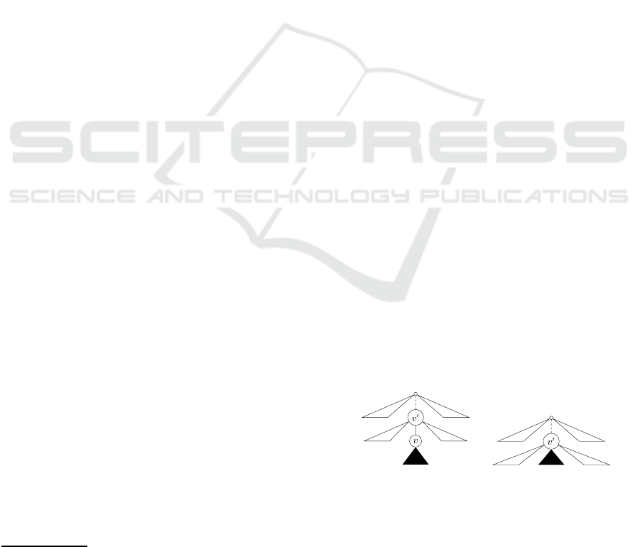
For a tree T and a vertex v ∈ T, the deletion of v
in T is to delete a non-root vertex v in T with a parent
v
′
, making the children of v become the children of
v
′
that are inserted in the place of v as a subset of the
children of v
′
. We denote the result of the deletion of
v in T by delete(T, v). See the following figure.
T delete(T,v)
Definition 3 (Inclusion). Let P and T be trees. We
sometimes call P a pattern tree and T a text tree.
Then, we say that P is an inclusion of T, denoted by
P ⊑ T, if either P
∼
=
T or there exists a sequence of
vertices v
1
,.. . , v
k
in T such that T
0
∼
=
T, T
k
∼
=
P and
T
i+1
∼
=
delete(T
i
,v
i+1
) (0 ≤ i ≤ k − 1).
Caterpillar Inclusion: Inclusion Problem for Rooted Labeled Caterpillars
281
We can characterize the tree inclusion by using the
following inclusion mapping (Hokazono et al., 2012),
which is a variant of a Tai mapping in the tree edit
distance (Tai, 1979).
Definition 4 (Inclusion mapping). Let P and T be
trees. Then, we say that the triple (I, P,T) is an
(unordered) inclusion mapping from P to T if I ⊆
V(P)×V(T) satisfies the conditions 1, 3 and 4 in Def-
inition 1, that is:
1. ∀v ∈ V(P)∃w ∈ V(T)
((v, w) ∈ I) ∧ (l(v) = l(w))
.
(inclusion condition)
2. ∀(v
1
,w
1
),(v
2
,w
2
) ∈ I
(v
1
= v
2
) ⇐⇒ (w
1
= w
2
)
.
(one-to-one condition)
3. ∀(v
1
,w
1
),(v
2
,w
2
) ∈ I
(v
1
≤ v
2
) ⇐⇒ (w
1
≤ w
2
)
.
(ancestor condition)
We will use I instead of (I, P,T) when there is no con-
fusion.
It is obvious that P ⊑ T if and only if there exists
an inclusion mapping from P to T, and P
∼
=
T if and
only if P ⊑ T and T ⊑ P.
Theorem 1. (Kilpel¨ainen and Mannila, 1995) For
trees P and T, the problem of determining whether or
not P ⊑ T is NP-complete. This statement also holds
even if the maximum height of T is at most 3.
4 CATERPILLAR INCLUSION
In this section, we investigate a caterpillar inclusion
as the inclusion such that both a pattern tree P and a
text tree T are caterpillars.
Let P and T be caterpillars such that r(P) = v
1
and r(T) = w
1
. Then, we denote bb(P) = [v
1
,.. . , v
n
]
for (v
i
,v
i+1
) ∈ E(P) and bb(T) = [w
1
,.. . , w
m
] for
(w
j
,w
j+1
) ∈ E(T). Also L
i
(resp., M
j
) denotes the set
of leaves that are children of v
i
(resp., w
j
) for 1 ≤ i ≤ n
(resp., 1 ≤ j ≤ m).
In this section, we use a multiset of labels in order
to compare two sets of vertices. A multiset on Σ is
a mapping S : Σ → N. For a multiset S on Σ, we say
that a ∈ Σ is an element of S if S(a) > 0. An empty
multiset is a multiset S such that S(a) = 0 for every
a ∈ Σ and denote it by
/
0 (like as a standard set). Let
S
1
and S
2
be multisets on Σ. Then, we define the inter-
section S
1
⊓ S
2
and the difference S
1
\ S
2
as multisets
satisfying that (S
1
⊓ S
2
)(a) = min{S
1
(a),S
2
(a)} and
(S
1
\ S
2
)(a) = max{S
1
(a)− S
2
(a),0} for every a ∈ Σ.
Note that S
1
\S
2
= S
1
\S
1
⊓S
2
. For a set V of vertices,
we denote the multiset of labels occurring in V by
e
V.
Then, we design the algorithm CATINC in Algo-
rithm 1.
procedure CATINC(P, T)
/ P : caterpillar, bb(P) = [v
1
,.. . , v
n
] /
/ T : caterpillar, bb(T) = [w
1
,.. . , w
m
] /
if n > m then return “No”; halt;1
else2
j ← 1;3
for i = 1 to n do4
while l(v
i
) 6= l(w
j
) do5
if j < m then j
++
;6
else return “No”; halt;7
/ l(v
i
) = l(w
j
) /
e
N
i
←
e
L
i
\
f
M
j
;8
while
(i < n and
e
N
i
6=
/
0) or
9
(i = n and
f
N
n
\
^
{w
j+1
} 6=
/
0)
do
if j < m then10
j
++
;
e
N
i
←
e
N
i
\
f
M
j
;11
else return “No”; halt;12
j
++
;13
return “Yes”;14
Algorithm 1: CATINC.
Example 1. Consider a pattern caterpillar P and a text
caterpillar T in Figure 1, where bb(P) = [v
1
,v
2
,v
3
]
and bb(T) = [w
1
,.. . , w
6
]. Also we denote a multiset
as a string, that is, we denote a multiset {a, a,b, c, c}
as a string a
2
bc
2
, for example. Then, we run the algo-
rithm CATINC(P,T).
First, the algorithm CATINC(P,T) finds w
j
such
that l(v
1
) = l(w
j
). Then, it sets j = 1 and computes
e
L
1
\
f
M
1
= bc\ b
2
= c =
f
N
1
. Since
f
N
1
6=
/
0, after in-
crementing j as 2 it computes
f
N
1
\
f
M
2
= c \ c
2
=
/
0,
which is set to
f
N
1
. Since
f
N
1
=
/
0, the algorithm
CATINC(P,T) increments j as 3 and i as 2.
Secondly, the algorithm CATINC(P,T) finds w
j
such that l(v
2
) = l(w
j
) for j ≥ 3. Then, it sets j = 3
and computes
e
L
2
\
f
M
3
= b
2
\ b
2
c =
/
0 =
f
N
2
. Since
f
N
2
=
/
0, the algorithm CATINC(P,T) increments j as
4 and i as 3.
Finally, the algorithm CATINC(P,T) finds w
j
such
that l(v
3
) = l(w
j
) for j ≥ 4. Then, it sets j = 4 and
computes
e
L
3
\
f
M
4
= c
3
\ b
2
c = c
2
=
f
N
3
. Since
f
N
3
6=
/
0, after incrementing j as 5 it computes
f
N
3
\
f
M
5
=
c
2
\ c = c, which is set to
f
N
3
. Since
f
N
3
6=
/
0, after
incrementing j as 6 it computes
f
N
3
\
f
M
6
= c \ bc =
ICPRAM 2022 - 11th International Conference on Pattern Recognition Applications and Methods
282

centering
a
v
1
b
c a
v
2
b b
a
v
3
c c c
a
w
1
b b b
a
w
2
c c c a
w
3
b b
c a
w
4
b b
c a
w
5
b
c a
w
6
b
c
P T
a
b
c a
b b
a
c c c
a
b b b
a
c c c a
b b
c a
b b
c a
b
c a
b
c
I
Figure 1: The pattern caterpillar P, the text caterpillar T and the inclusion mapping I from P to T in Example 1.
/
0, which is set to
f
N
3
. Since
f
N
3
=
/
0, the algorithm
CATINC(P,T) returns “Yes”.
We can obtain the inclusion mapping I from P to
T consisting of the pairs (v
1
,w
1
),(v
2
,w
3
),(v
3
,w
4
) for
backbones such that l(v
i
) = l(w
j
) at line 5, the cor-
respondences between
e
L
i
and
f
M
j
in line 8 such that
e
L
i
⊓
f
M
j
and the correspondences between
e
N
i
and
f
M
j
in line 10 such that
e
N
i
⊓
f
M
j
. Figure 1 illustrates the
inclusion mapping I as the dashed line obtained by
applying the algorithm CATINC(P, T).
Then, we can obtain the following main theorem
of this paper.
Theorem 2. Let P and T be caterpillars, where h =
h(P), H = h(T) and σ = |Σ|. Then, we can determine
whether or not P ⊑ T in O((h+ H)σ) time.
Proof. First, we showthe correctness of the algorithm
CATINC. Let i be a current index in the for-loop of the
algorithm CATINC. Also suppose that I is a mapping
from P to T implicitly obtained by CATINC returned
to “Yes.”
Then, CATINC first finds j such that l(v
i
) = l(w
j
)
for v
i
∈ bb(P) and w
j
∈ bb(T), which implies that
(v
i
,w
j
) ∈ I. Next, for i and j, CATINC corresponds
the leaves in L
i
to the leaves in M
j
as possible, where
the corresponding pair (v, w) ∈ L
i
× M
j
are added to
I, and then store the remained (non-mapped) labels of
leaves in
e
L
i
as
e
N
i
, which is realized as the line 8. Then,
until
e
N
i
is empty, CATINC increments j and finds the
corresponding leaves in the next set M
j
of leaves in T
to N
i
, where the found pair (v, w) ∈ N
i
× M
j
is added
to I. Finally, when i = n, the condition in while-loop
is changed that
f
N
n
∪
^
{w
j+1
} is empty. This means
that, when
f
N
n
6=
/
0 and
f
N
n
\
^
{w
j+1
} =
/
0, at most one
vertex w
j+1
∈ bb(T) is corresponding to a leaf v ∈ L
n
and (v,w
j+1
) is implicitly added to I. In this case, the
algorithm CATINC finishes and there exists no pair
(v, w) ∈ I such that w is a descendant of w
j+1
.
For the obtained mapping I by the algorithm CAT-
INC, it is obvious that I satisfies the inclusion con-
dition and the one-to-one condition. Also, for pairs
(v
i
,w
j
),(v
i+1
,w
k
) ∈ I such that v
i
,v
i+1
∈ bb(P) and
w
j
,w
k
∈ bb(T) (1 ≤ i < n − 1, 1 ≤ j < k ≤ m), every
leaf in L
i
is corresponding to a leaf in M
j
∪···∪M
k−1
.
In other words, there exist no pairs (v,w),(v
′
,w
′
) ∈ I
such that v ∈ L
i
, w ∈ M
j
, v
′
∈ L
i
′
, w
′
∈ M
j
′
, i < i
′
and
j
′
< j. Furthermore, for i = n, let I
n
= {(v, w) ∈ I |
v ∈ L
n
}. Note that at most one vertex w
j+1
∈ bb(T)
is corresponding to a leaf in L
n
. If such a w
j+1
ex-
ists, then there exists no pair (v,w) ∈ I
n
such that w
is a descendant of w
j+1
. This implies that neither w
is an ancestor of w
′
nor w
′
is an ancestor of w for ev-
ery w and w
′
such that w 6= w
′
and (v, w), (v
′
,w
′
) ∈ I
n
.
Then, I satisfies the ancestor condition. Hence, I is an
inclusion mapping from P to T.
Next, we show the time complexity of the algo-
Caterpillar Inclusion: Inclusion Problem for Rooted Labeled Caterpillars
283

rithm CATINC. By using the hash table of Σ, we
can process
e
N
i
←
e
L
i
\
f
M
j
and
e
N
i
←
e
N
i
\
f
M
j
in O(σ)
time. Also we can determine whether or not
e
N
i
6=
/
0
in O(σ) time. Furthermore, j changes from 1 to m in
the for-loop while i changes from 1 to n in CATINC.
Since n = h and m = H, the algorithm CATINC runs
in O((h+ H)σ) time.
Theorem 2 also claims that the structural restric-
tion of caterpillars provides the limitation of tractabil-
ity of the tree inclusion problem. We say that a tree
is a generalized caterpillar if it is transformed to a
caterpillar after removing all the leaves in it. Then,
Theorem 1 implies the following theorem.
Theorem 3. (Kilpel¨ainen and Mannila, 1995) Let P
be a caterpillar and T a generalizedcaterpillar. Then,
the problem of determining whether or not P ⊑ T is
NP-complete. This statement also holds even if the
maximum height of T is at most 3.
Theorem 3 is similar that the structural restriction
of caterpillars provides the limitation of tractability
of computing the edit distance. Whereas the prob-
lem of computing the edit distance between caterpil-
lars is tractable as stated in Section 1, the problem
of computing the edit distance between generalized
caterpillars is MAX SNP-hard. This statement also
holds even if the maximum height is at most 3 or the
cost function is the unit cost function (Muraka et al.,
2018).
5 EXPERIMENTAL RESULTS
In this section, we give the experimental results of
computing CATINC. Here, the computer environment
is that OS is Ubuntu 18.04.4, CPU is Intel Xeon E5-
1650 v3(3.50GHz) and RAM is 3.8GB.
We deal with caterpillars for N-glycans and all-
glycans from KEGG
4
, CSLOGS
5
, the largest 5,154
caterpillars (0.1%) in dblp
6
(refer to dblp
0.1%
), Swis-
sProt and non-isomorphic caterpillars in TPC-H (re-
fer to TPC-H
◦
) from UW XML Repository
7
. Also
we deal with caterpillars obtained by deleting the root
in Auction (refer to Auction
−
) and non-isomorphic
caterpillars obtained by deleting the root in Nasa (re-
fer to NASA
−
◦
), Protein (refer to Protein
−
◦
) and Uni-
4
Kyoto Encyclopedia of Genes and Genomes,
http://www.kegg.jp/
5
http://www.cs.rpi.edu/˜zaki/www-
new/pmwiki.php/Software/Software
6
http://dblp.uni-trier.de/
7
http://aiweb.cs.washington.edu/research/projects/xmltk/
xmldata/www/repository.html
versity (refer to University
−
◦
) from UW XML Reposi-
tory. Table 1 illustrates the information of such cater-
pillars. Here, #, n, d, h, λ and β are the number of
caterpillars, the average number of vertices, the aver-
age degree, the average height, the average number of
leaves and the average number of labels.
Table 1: The information of caterpillars.
data # n d h λ β
N-glycans 514 6.40 1.84 4.22 2.18 4.50
all-glycans 7,984 4.74 1.49 3.02 1.72 2.84
CSLOGS 41,592 5.84 3.05 2.20 3.64 5.18
dblp
0.1%
5,154 41.74 40.73 1.01 40.73 10.61
SwissProt 6,804 35.10 24.96 2.00 33.10 16.79
TPC-H
◦
8 8.63 7.63 1.00 7.63 8.63
Auction
−
259 4.29 3.00 0.71 3.57 4.29
Nasa
−
◦
33 7.27 5.15 1.64 5.64 3.18
Protein
−
◦
5,150 4,97 3.63 1.16 3.81 4.57
University
−
◦
26 1.35 0.35 0.19 1.15 1.35
We compare all the pairs (P, T) in the caterpillars
in Table 1. The number of pairs is # × (# − 1), and
Table 2 summarizes such number as #pairs.
Table 2: The number (#pairs) of all the pairs in caterpillars
in Table 1.
data #pairs
N-glycans 263,682
all-glycans 63,736,272
CSLOGS 1,729,852,872
dblp
0.1%
26,558,562
SwissProt 46,287,612
data #pairs
TPC-H
◦
56
Auction
−
66,822
Nasa
−
◦
1,056
Protein
−
◦
26,517,350
University
−
◦
650
Table 3 illustrates the number (#pairs) of pairs
(P, T) such that P ⊑ T with its ratio (%) in all the
pairs, and the total and average running time. Note
that we just apply the algorithm CATINC to all the
pairs without pruning by the number of vertices, and
so on.
Table 3 shows that Auction
−
has the largest ra-
tio of 13.95% in all the data, and the ratio of Nasa
−
◦
is also more than 10%. One of the reason is that their
data are obtained by deleting the root and the caterpil-
lars as the children of the root have similar structures.
On the other hand, Table 3 also shows that Swis-
sProt has the largest average running time in all the
data, which is more than twice to the average running
time of the other data. Also, dblp
0.1%
has the sec-
ond largest average running time. One of the reason
that the caterpillars in SwissProt and dblp
0.1%
have
the larger degree and the larger number of leaves than
the other data.
ICPRAM 2022 - 11th International Conference on Pattern Recognition Applications and Methods
284

Table 3: The number (#pairs) of pairs (P, T) such that P⊑ T
with its ratio (%) in all the pairs, the total running time (sec)
and average running time (msec).
data #pairs % total ave.
(sec) (msec)
N-glycans 8,773 3.33 15.980 0.0603
all-glycans 704,521 1.11 2,252.321 0.0353
CSLOGS 2,070,110 0.12 83,961.780 0.0485
dblp
0.1%
1,855,880 6.99 2,045.844 0.0770
SwissProt 1,400,455 3.03 7,440.401 0.1607
TPC-H
◦
0 0 0.004 0.0714
Auction
−
9,324 13.95 1.728 0.0259
Nasa
−
◦
108 10.23 0.030 0.0284
Protein
−
◦
3,701 0.01 587.739 0.0222
University
−
◦
1 0.15 0.006 0.0092
Next, we investigate how many caterpillars are in-
cluded in another caterpillar in the set of caterpillars.
Let D be the set of caterpillars. For P ∈ D, we call the
number of text caterpillars in D which includes P the
inclusion number of P in D and denote it by inc
D
(P).
Furthermore, we define the following formulas.
h
inc(k, D) = |{P ∈ D | inc
D
(P) = k}|,
maxinc(D) = max{inc
D
(P) | P ∈ D},
pat(D) =
maxinc(D)
∑
k=1
h
inc(k, D),
ratio(D) =
pat(D)
|D|
.
Since every pattern caterpillar P having T ∈ D
such that P ⊑ T is counted just once in pat(D) for
D, pat(D) is the number of caterpillars in D included
in some caterpillar (without themselves) in D. Then,
ratio(D) is the ratio of such caterpillars in D.
Tables 4, 5 and 6 illustrate the histograms of
h
inc(k, D) with maxinc(D), pat(D) and ratio(D)
for every D. Here, since Auction
−
, Nasa
−
◦
and
University
−
◦
have particular distributions, we summa-
rize them as Table 6.
Tables 4 and 5 (except Table 6) show that Swis-
sProt has the largest value of maxinc in all the data.
Also, all-glycans has the larger value of maxinc
than CSLOGS and dblp
0.1%
, whereas all-glycans
has the much smaller value of “#pairs” in Table 3
than CSLOGS and dblp
0.1%
. Furthermore, whereas
CSLOGS has the largest value of pat, it also has the
largest value of “#” in Table 1 and “#pairs” in Table 3.
On the other hand, dblp
0.1%
has the largest value of
ratio and SwissProt has the second largest value of
ratio over 90%.
Hence, we conjecture that the values of maxinc
and ratio are independent from the value of inc and
depend on the forms of caterpillars in data.
Table 4: The histograms of h
inc(k, D) with maxinc(D),
pat(D) and ratio(D) (%) for N-glycans, all-glycans and
CSLOGS.
N-glycans all-glycans CSLOGS
k h inc(k, D)
1 69
2 33
3 20
4 22
5 11
6 16
7 16
8 16
9 8
10 9
≥ 11 174
220 maxinc
394 pat
76.65 ratio (%)
k h inc(k, D)
1 681
2 462
3 370
4 275
5 184
6 209
7 154
8 167
9 119
10 127
≥ 11 4,105
2,938 maxinc
6,853 pat
85.83 ratio (%)
k h inc(k, D)
1 4,772
2 2,377
3 1,524
4 1,038
5 884
6 641
7 534
8 454
9 429
10 330
≥ 11 13,215
1,702 maxinc
26,198 pat
62.99 ratio (%)
Table 5: The histograms of h inc(k,D) with maxinc(D),
pat(D) and ratio(D) (%) for dblp
0.1%
, SwissProt and
Protein
−
◦
.
dblp
0.1%
SwissProt Protein
−
◦
k h inc(k, D)
1 42
2 38
3 32
4 29
5 34
6 26
7 27
8 26
9 25
10 19
≥ 11 4,794
1,939 maxinc
5,092 pat
98.80 ratio (%)
k h inc(k, D)
1 361
2 250
3 202
4 166
5 153
6 141
7 101
8 98
9 85
10 116
≥ 11 4,488
5,666 maxinc
6,161 pat
90.55 ratio (%)
k h inc(k, D)
1 494
2 43
3 28
4 26
5 17
6 12
7 16
8 15
9 10
10 8
≥ 11 93
149 maxinc
762 pat
14.80 ratio (%)
Finally, we give the examples of a pattern cater-
pillar P and a text caterpillar T such that inc
D
(P) = 1.
for several data D.
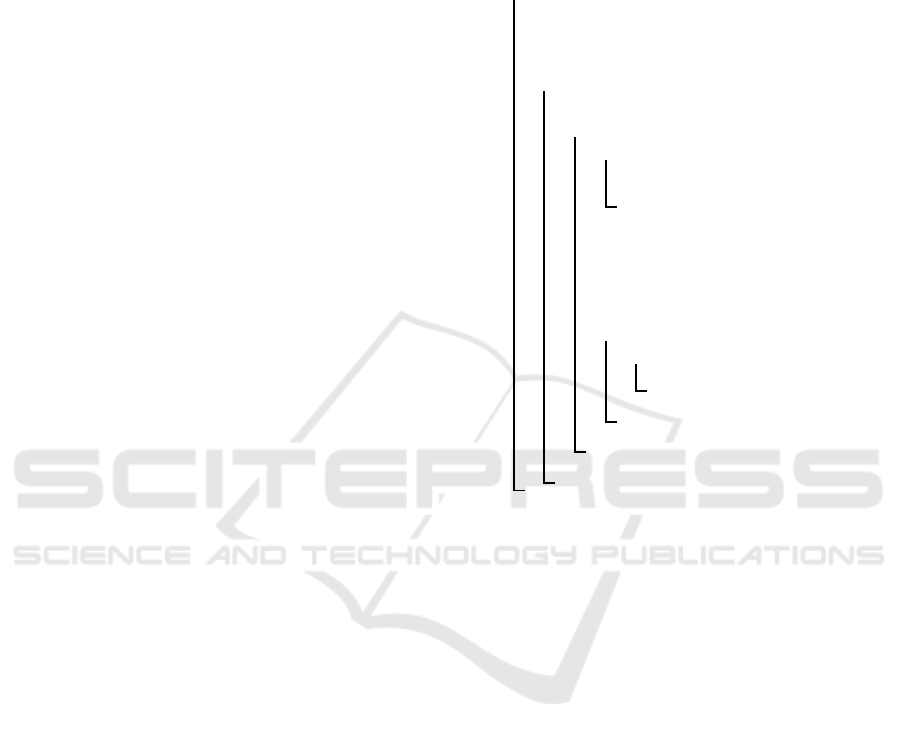
Figure 2 illustrates an example of P = G00954 and
T = G04792 in N-glycans. Also Figure 3 illustrates
an example of P = G10338 and T = G10334 in all-
glycans.
On the other hand, Figure 4 illustrates an exam-
ple of P = CL33073 and T = CL30743 in CSLOGS.
Furthermore, Figure 5 illustrates an example of P =
ID-T10728
005 and T = ID-T33084 006 in Protein
−
◦
.
Caterpillar Inclusion: Inclusion Problem for Rooted Labeled Caterpillars
285
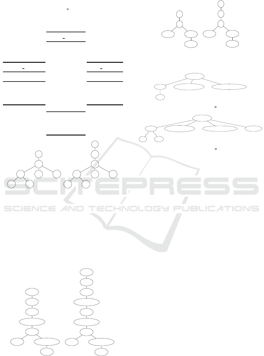
Table 6: The histograms of h inc(k, D) with maxinc(D),
pat(D) and ratio(D) (%) for Auction
−
, Nasa
−
◦
and
University
−
◦
.
Auction
−
Nasa
−
◦
University
−
◦
k h inc(k, D)
36 259
36 maxinc
259 pat
100.00 ratio (%)
k h inc(k, D)
1 5
2 3
3 3
4 2
5 2
6 2
7 2
8 2
9 2
10 1
10 maxinc
24 pat
72.73 ratio (%)
k h inc(k, D)
1 1
1 maxinc
1 pat
3.85 ratio (%)
I
C
D
D D
B D
I
B
C
D
D D
B D
P = G10338 T = G10334
Figure 2: P and T in N-glycans.
6 CONCLUSION
In this paper, we have designed the algorithm CATINC
to determine whether or not P ⊑ T in O((h+ H)σ)
time, where h is the height of P, H is the height of
T and σ is the number of labels occurring in P and
Cer
Glc
Gal
GlcNAc
Gal
Fuc GlcNAc
Gal
Cer
Glc
Gal
GlcNAc
Gal
GlcNAc
Gal
Fuc GlcNAc
Gal
P = G00057 T = G00073
Figure 3: P and T in all-glycans.
1
7
105 106
633
1
5
7
105 106
633
P = CL33073 T = CL00501
Figure 4: P and T in CSLOGS.
genetics
gene
uid
map-position
mobile-element
P = ID-T10728 005
genetics
gene
db uid
map-position
mobile-element
introns
T = ID-T33084 006
Figure 5: P and T in Protein
−
◦
.
T. Also, we have given experimental results for the
algorithm CATINC by using real caterpillar data.
Note that the algorithm CATINC just determines
whether or not P ⊑ T but does not count the number
of matching positions when P ⊑ T. Then, it is a future
work to improve the algorithm CATINC to store the
matching positions and count them. Here, it is nec-
essary to count the correspondence between multisets
of labels in leaves carefully.
Since the tree inclusion is NP-complete, it is also
a future work to introduce the heuristic algorithm by
incorporating the algorithm CATINC with the heavy
caterpillar of trees such as (Abe et al., 2020), for ex-
ample.
REFERENCES
Abe, N., Yoshino, T., and Hirata, K. (2020). Heavy cater-
pillar distance for rooted labeled unordered trees. In
Proc. ICPRAM’20, pages 198–204.
Akutsu, T., Fukagawa, D., Halld´orsson, M. M., Takasu, A.,
and Tanaka, K. (2013). Approximation and parame-
terized algorithms for common subtrees and edit dis-
tance between unordered trees. Theoret. Comput. Sci.,
470:10–22.
Akutsu, T., Jansson, J., Li, R., Takasu, A., and Tamura, T.
(2021). New and improved algorithms for unordered
tree inclusion. Theoret. Comput. Sci., 883:83–98.
Gallian, J. A. (2007). A dynamic survey of graph labeling.
Electorn. J. Combin., 14:DS6.
Hirata, K., Yamamoto, Y., and Kuboyama, T. (2011). Im-
ICPRAM 2022 - 11th International Conference on Pattern Recognition Applications and Methods
286

proved MAX SNP-hard results for finding an edit dis-
tance between unordered trees. In Proc. CPM’11
(LNCS 6661), pages 402–415.
Hokazono, T., Kan, T., Yamamoto, Y., and Hirata, K.
(2012). An isolated-subtree inclusion for unordered
trees. In Proc. IIAI AAI ’12, pages 345–350.
Kilpel¨ainen, P. and Mannila, H. (1995). Ordered and un-
ordered tree inclusion. SIAM J. Comput., 24:340–356.
Matou˘sek, J. and Thomas, R. (1992). On the complexity of
finding iso- and other morphisms for partial k-trees.
Discrete Math., 108:343–364.
Muraka, K., Yoshino, T., and Hirata, K. (2018). Computing
edit distance between rooted labeled caterpillars. In
Proc. FedCSIS’18, pages 245–252.
Shamir, R. and Tsur, D. (1999). Faster subtree isomor-
phism. Algorithmica, 33:267–280.
Tai, K.-C. (1979). The tree-to-tree correction problem. J.
ACM, 26:422–433.
Ukita, Y., Yoshino, T., and Hirata, K. (2021). Caterpil-
lar alignment distance for rooted labeled caterpillars:
Distance based on alignments required to be caterpil-
lars. In Recent advance in computational optimiza-
tion, pages 111–134.
Valiente, G. (2002). Algorithms on trees and graphs.
Springer.
Valiente, G. (2005). Constrained tree inclusion. J. Discrete
Algorithms, 3:431–447.
Zhang, K. and Jiang, T. (1994). Some MAX SNP-hard re-
sults concerning unordered labeled trees. Inform. Pro-
cess. Lett., 49:249–254.
Zhang, K., Wang, J., and Shasha, D. (1996). On the editing
distance between undirected acyclic graphs. Internat.
J. Found. Comput. Sci., 7:43–58.
Caterpillar Inclusion: Inclusion Problem for Rooted Labeled Caterpillars
287
