On the Suitability of SHAP Explanations for Reﬁning Classiﬁcations

Yusuf Arslan

1 a

, Bertrand Lebichot

1 b

, Kevin Allix

1 c

, Lisa Veiber

1 d

, Cl

ement Lefebvre

Andrey Boytsov

2 e

, Anne Goujon

, Tegawend

e Bissyande

1 f

and Jacques Klein

1 g

University of Luxembourg, Luxembourg

BGL BNP Paribas, Luxembourg

Keywords:

SHAP Explanations, Shapley Values, Explainable Machine Learning, Clustering, Rule Mining.

Abstract:

In industrial contexts, when an ML model classiﬁes a sample as positive, it raises an alarm, which is sub-

sequently sent to human analysts for veriﬁcation. Reducing the number of false alarms upstream in an ML

pipeline is paramount to reduce the workload of experts while increasing customers’ trust. Increasingly, SHAP

Explanations are leveraged to facilitate manual analysis. Because they have been shown to be useful to human

analysts in the detection of false positives, we postulate that SHAP Explanations may provide a means to auto-

mate false-positive reduction. To conﬁrm our intuition, we evaluate clustering and rules detection metrics with

ground truth labels to understand the utility of SHAP Explanations to discriminate false positives from true

positives. We show that SHAP Explanations are indeed relevant in discriminating samples and are a relevant

candidate to automate ML tasks and help to detect and reduce false-positive results.

1 INTRODUCTION

Machine Learning (ML) is increasingly explored in

industrial settings to automate a variety of decision-

making processes (McKinsey, 2019). In Fin-

Tech (Gomber et al., 2018), ML models are leveraged

to scale the identiﬁcation of fraudulent transactions.

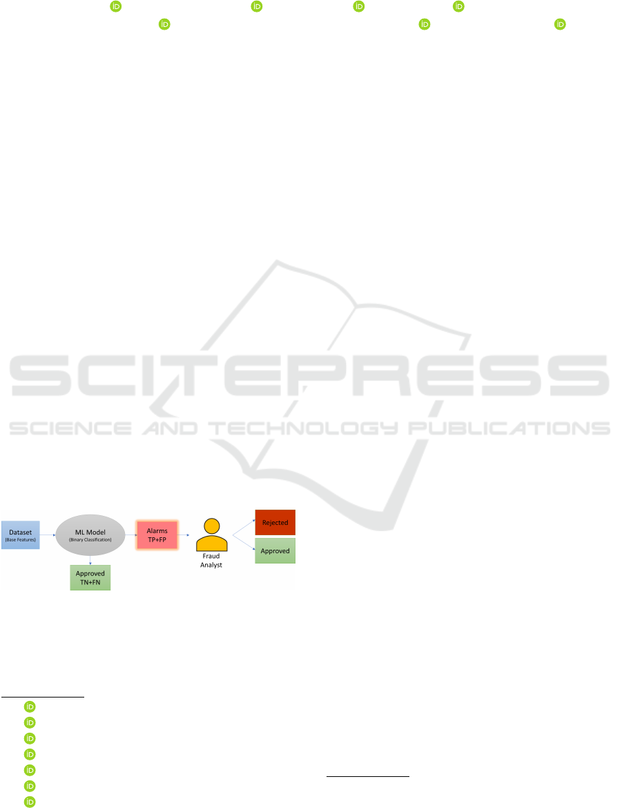
Unfortunately, an ML model is not an oracle: when

it raises an alarm, human analysts are still often re-

quired to double-check (Ghamizi et al., 2020). This

process can be seen in Figure 1.

Figure 1: Alarm Processing with Human Intervention.

Enabling practitioners to readily identify false

positives among ML model classiﬁcations has be-

come paramount to facilitate integration in indus-

trial settings. Given the high cost of manual triag-

https://orcid.org/0000-0003-4423-4725

https://orcid.org/0000-0003-2188-0118

https://orcid.org/0000-0003-3221-7266

https://orcid.org/0000-0002-3692-8308

https://orcid.org/0000-0003-1166-5908

https://orcid.org/0000-0001-7270-9869

https://orcid.org/0000-0003-4052-475X

ing (Wedge et al., 2018) and the risk of losing

customer trust (Pascual et al., 2015), practitioners

are seeking tool support in their veriﬁcation tasks.

In this context, model explanations constitute the

main instrument that is made available to practition-

ers. SHapley Additive exPlanations (SHAP

) (Lund-

berg and Lee, 2017), for example, have already

been proven useful to triage false positives. SHAP

computes feature contributions, called SHAP values,

which are used to explain why a given prediction has

been made or how the model behaves.

Consider the Adult dataset

where the goal is to

predict the income of adult individuals: is a person

making more than $50k a year or not. We build

an ML model based on the enumerated features in

the dataset and with Gradient Boosting as a learner,

which yielded a False Positive rate of 10%. A hu-

man analyst can quickly suspect a false positive given

the contributions of the different features in the pre-

diction: obvious outliers can be spotted based on

domain expertise. In a recent work, it has been

shown that SHAP Explanations can indeed help do-

main experts effectively—although manually—triage

false positives (Weerts, 2019). Our postulate in this

study is that if it works with humans, it could work

with algorithms. Indeed, if humans are able to lever-

age information in SHAP explanations, such infor-

mation may be automatically and systematically ex-

https://github.com/slundberg/shap

https://archive.ics.uci.edu/ml/datasets/adult

Arslan, Y., Lebichot, B., Allix, K., Veiber, L., Lefebvre, C., Boytsov, A., Goujon, A., Bissyande, T. and Klein, J.

On the Suitability of SHAP Explanations for Reﬁning Classiﬁcations.

DOI: 10.5220/0010827700003116

In Proceedings of the 14th International Conference on Agents and Artiﬁcial Intelligence (ICAART 2022) - Volume 3, pages 395-402

ISBN: 978-989-758-547-0; ISSN: 2184-433X

395

ploited in an automated setting.

This paper. Our study considers the problem of

false positives identiﬁcation in ML classiﬁcation. We

assume that a classiﬁer was trained for a certain task,

and we seek to identify false positives to increase

the dependability of the overall process. Concretely,

we investigate the potential of SHAP Explanations

to be used in an automated pipeline for discriminat-

ing false-positive (FP) and true-positive (TP) samples.

This paper is a ﬁrst empirical analysis where we pro-

pose to evaluate the added-value of SHAP explana-

tions compared to the features that were available for

the classiﬁcation. We will refer to those available fea-

tures as base features in this paper. The features ob-

tained through SHAP explanations will be referred to

as SHAP features. Notice that SHAP, for each sam-

ple, provides a ﬂoat per feature, and the full set of

SHAP features have the same size as the full set of

base features.

To perform our empirical analysis where we inves-

tigate the added-value of SHAP features for FP detec-

tion, we ﬁrst explore the TP samples and FP samples

with respect to SHAP explanations, which is evalu-

ated in clustering experiments. The idea is that the

purity of the clusters can help us assess the predictive

power of SHAP features. We will also investigate rule

extraction as another method to uncover the potential

of SHAP features to detect FPs. More precisely, our

study explores the following research questions:

RQ 1: Do SHAP features and base features bring dif-

ferences in terms of the number of clusters?

RQ 2: Do SHAP features provide relevant informa-

tion, from a clustering point of view, that could be

leveraged to distinguish FP and TP, compared to base

features?

RQ 3: Do SHAP features provide relevant informa-

tion, from a rules extraction point of view, that could

be leveraged to distinguish FP and TP, compared to

base features?

Overall we show that local explanations by SHAP,

which already help domain experts on ML decisions,

can be helpful to automate the detection of FPs and

TPs.

2 BACKGROUND AND RELATED

WORK

With the advancement of technology, AI and ML have

become ubiquitous in many domains (Veiber et al.,

2020). The necessity of explaining the decision mech-

anism of AI and ML models increases with their pop-

ularity as well (Hind et al., 2019). The Explain-

able Artiﬁcial Intelligence (XAI) domain is the re-

sult of this necessity and has become a popular re-

search ﬁeld, including but not limited to marketing,

health, energy, and ﬁnance (Rai, 2020; Fellous et al.,

2019; Kuzlu et al., 2020; Veiber et al., 2020). How-

ever, the ﬁnancial domain has pre-requisites like fair-

ness (Goodman and Flaxman, 2017), which is im-

portant for XAI as well (Mueller et al., 2019). The

popular SHAP Explanation method (Lundberg and

Lee, 2017) attempts to solve the fairness issue in ex-

plainable ML using a popular game theory approach,

namely, Shapley Values (Shapley, 1953). SHAP Ex-

planations ensure a fair evaluation of features (Mol-

nar, 2020) and output feature contribution as SHAP

Values. SHAP is widely used in the ﬁnancial domain

for various projects (Bracke et al., 2019; Mokhtari

et al., 2019; Bhatt et al., 2020)

Lin (Lin, 2018) evaluates SHAP and Lo-

cal Interpretable Model-agnostic Explanations

(LIME)

(Ribeiro et al., 2016) to obtain useful

information for domain experts and facilitate the FP

reduction task. Lin (Lin, 2018) suggests eliminating

FPs by employing an ML ﬁlter that uses SHAP

features instead of base features. According to their

ﬁndings, the performance of the ML ﬁlter using

SHAP features are better than the ML model using

base features and thus can be leveraged (Lin, 2018).

Weerts et al. (Weerts et al., 2019) test the useful-

ness of SHAP Explanations with real human users.

They consider SHAP Explanations as a decision sup-

port tool for domain experts. According to their ﬁnd-

ings, SHAP Explanations affects the decision-making

process of domain experts (Weerts, 2019).

Our study differs from the existing literature by

focusing on clustering and rule mining techniques to

present objective quantitative metrics with no human

experiments. We focus on clustering with the idea that

if FPs form coherent clusters (and TPs as well), then

SHAP features have the potential to be used to dis-

criminate FP and TP samples. Our idea here is that if

this is the case, it means FPs and TPs will be easier to

identify than with base features. Likewise, we focus

on rule mining with the idea that if high-quality rules

are obtained for FPs (and TPs as well), then SHAP

features have the potential to be used to discriminate

FP and TP samples.

2.1 Shapley Values

Shapley values (Shapley, 1953) derive from the coop-

erative game theory domain and have been inﬂuen-

tial in various domains for a long time (Quigley and

Walls, 2007; Sheng et al., 2016). In our case, the

values will produce an explanation which will sub-

https://github.com/marcotcr/lime

ICAART 2022 - 14th International Conference on Agents and Artiﬁcial Intelligence

396

sequently be used to detect FPs and TPs. The Shap-

ley values method satisﬁes the properties of symmetry

(interchangeable players should receive the same pay-

offs), dummy (dummy players should receive noth-

ing), and additivity (if the game is separated, so are

pay-offs) (Molnar, 2020). SHAP Explanations are al-

ready used in the ﬁnance sector (Hadji Misheva et al.,

2021), and these properties of SHAP are the reason

why it managed to gather some trust in this industry.

Moreover, SHAP explanations have been shown to

work well with the needs of ﬁnance actors (Hadji Mi-

sheva et al., 2021).

In our case, these properties do not ensure that the

separation power of Shapley values will be sufﬁcient

to discriminate FPs and TPs. Preliminary works (see

section 2), however, suggest this discriminative power

is often sufﬁcient in practice.

For the actual computation of the Shapley values,

we used the well-known SHAP package (Lundberg

and Lee, 2017).

2.2 SHAP as a Transformation of the

Learning Space

Let n

be the number of features and n

the number

of samples of our database. SHAP values can be seen

as the result of a (nonlinear) transformation f of the

learning space: f : R

×n

→ R

×n

. Indeed, each n

sample will receive n

SHAP values.

The idea is to use this transformation to send the

data to a more separable space. This idea is one of

the cornerstone of SVM and is widely used in many

domains (Shachar et al., 2018; Becker et al., 2019;

Song et al., 2013).

Examples of this transformation can be found in

Figure 2. In Figure 2, we used UMAP visualization, a

nonlinear dimensionality reduction technique, which

is becoming more popular than the classic PCA. On

this ﬁgure, with SHAP features, FPs are grouped to-

gether in a smaller number of areas with a high den-

sity of FPs, whereas with base features, they are more

scattered and intertwined with TPs.

2.3 Rule Mining by Subgroup Discovery

Subgroup Discovery (Kl

osgen, 1996) is one of the

popular data mining and machine learning techniques.

It reveals associations between samples with high

generality and distributional unusualness from a prop-

erty of interest (Helal, 2016; Lemmerich et al., 2013;

Imparato, 2013).

Subgroup Discovery lies at the intersection of

classiﬁcation and clustering (Helal, 2016). Subgroup

Discovery differs from clustering by searching rela-

tions with respect to a property of interest, while clus-

tering extracts the relation between unlabeled sam-

ples (Helal, 2016). The goal of the classiﬁcation is

to prepare a model with rules representing class char-

acteristics based on training samples, while Subgroup

Discovery extracts relations from a property of inter-

est (Helal, 2016).

Subgroup Discovery extracts relations with inter-

esting characteristics in the form of rules (Herrera

et al., 2011). Rules contain subgroup descriptions.

A rule (R) can be formally deﬁned as follows (Lavra

et al., 2004):

R : Cond → Target

value

(1)

where Cond is the conjunction of features and the

Target

value

is the value of the target variable for sub-

group discovery.

In this study, we use a publicly available Python

package for rule mining by subgroup discovery

3 EXPERIMENTAL SETUP

Following the idea that we search to automatize the

alarm processing pipeline, an initial classiﬁer is built

using the base features on a given dataset. Then, we

apply SHAP to explain the classiﬁcation outputs and

obtain the SHAP features. These features are then as-

sessed in this study through clustering and rule min-

ing experiments that measure to what extent they can

help discriminate true positives from false positives.

This process can be seen in Figure 3.

In this section, we describe the experimental

setup, metrics, and the datasets we used. To run our

experiments, we initially considered four ML classi-

ﬁcation algorithms, namely, Gradient Boosting Clas-

siﬁer (GBC), Balanced Bagging Classiﬁer, Balanced

Random Forest, and Balanced Easy Ensemble. The

best hyper-parameters for each classiﬁer are selected

by an extensive grid search using cross-validation (re-

sults are not reported here). Performance results of

classiﬁers are obtained by using stratiﬁed 5-fold 20-

repeats cross-validation. Eventually, we opted for

GBC since it gives the best results on these datasets.

We check the answers to each research question by

using 10-fold cross-validation.

3.1 Metrics

In this study, we report our clustering and rule mining

experiments using some metrics introduced here:

https://github.com/ﬂemmerich/pysubgroup

On the Suitability of SHAP Explanations for Reﬁning Classiﬁcations

397

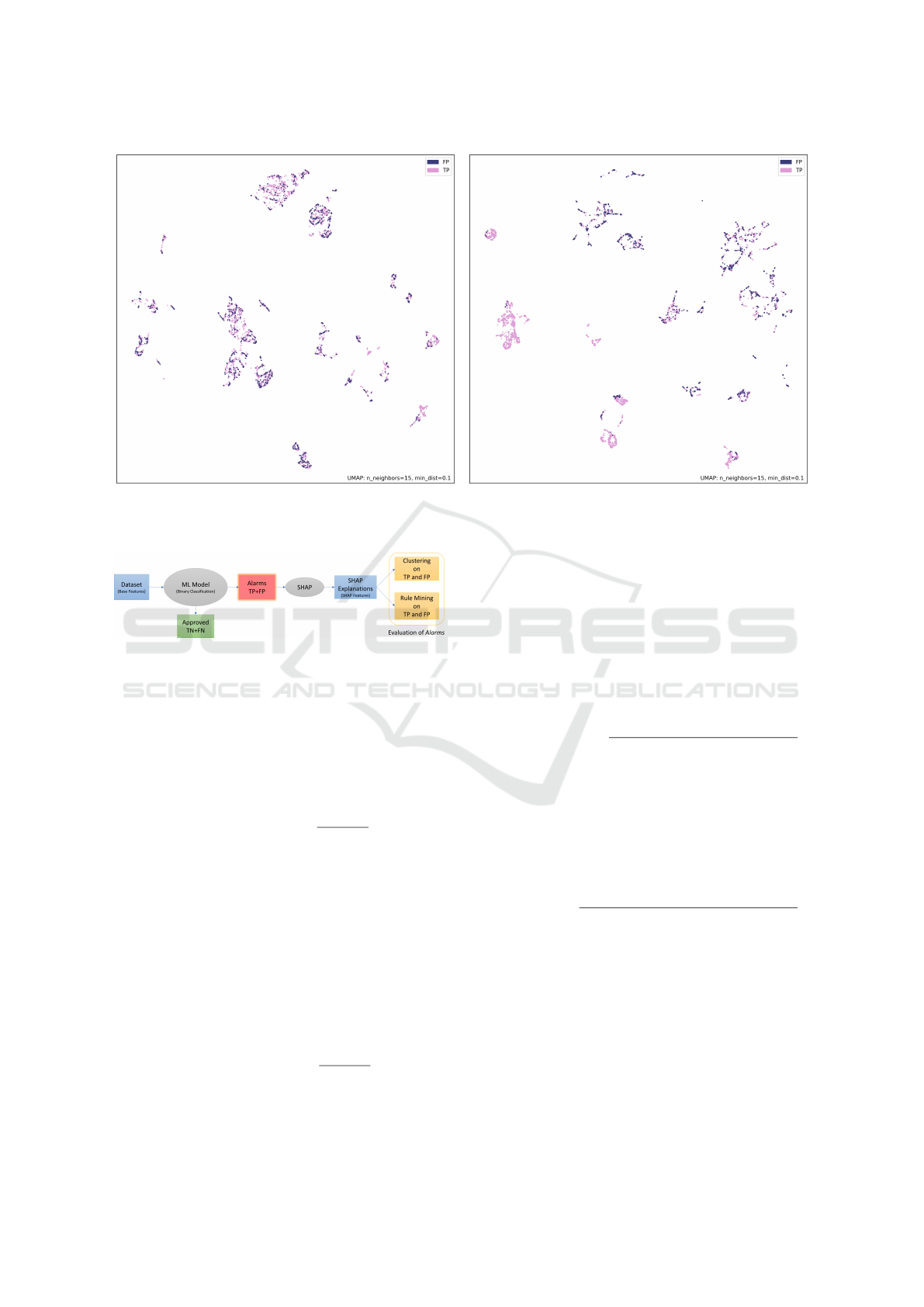
(a) Base Features (b) SHAP Features

Figure 2: UMAP of False and True Positives on Adult dataset with Base and SHAP features.

Figure 3: Our pipeline for Alarm Processing.

Homogeneity: A perfectly homogeneous clus-

tering is achieved when each cluster is only com-

posed of a sample from the class label (Rosenberg and

Hirschberg, 2007). In this study, we use homogeneity

to measure the similarity within clusters in terms of

FPs and TPs. Homogeneity can be expressed by the

following formula:

Homogeneity = 1 −

H(C |G)

H(C , G)

(2)

where C is a cluster, G is a class, H(C|G) is the condi-

tional entropy of the classes given the cluster assign-

ments, and H(C, G) is the joint entropy for normal-

ization (Utt et al., 2014).

Completeness: A clustering result achieved perfect

completeness if all the data points which are mem-

bers of a given class are elements of the same clus-

ter (Rosenberg and Hirschberg, 2007). In this study,

we use completeness to assess whether all FPs or TPs

are assigned to the same clusters. Completeness is

deﬁned as:

Completeness = 1 −

H(G|C)

H(G, C)

(3)

where C is a cluster, G is a class, H(G|C) is the con-

ditional entropy of clusters given class, and H(G, C)

is the entropy of the classes (Utt et al., 2014).

V-measure: V-measure is the harmonic mean

of homogeneity and completeness scores (Rosen-

berg and Hirschberg, 2007). In this study, we

use v-measure to check the validity (Rosenberg and

Hirschberg, 2007) of the cluster, which quantiﬁes

cluster concentration and inter-cluster separation, of

clustering algorithm with respect to homogeneity and

completeness. V-measure is deﬁned as:

V −measure = 2 ×

Homogeneity ×Completeness

Homogeneity +Completeness

(4)

Adjusted Mutual Information (AMI): AMI mea-

sures the agreement between clustering and the

ground truth (Vinh et al., 2010). AMI is 1.0 when

two partitions are identical, disregarding permuta-

tions. AMI can be expressed for two clusterings U

and V , by the following formula:

AMI(U, V ) =

[MI(U, V ) −E(MI(U, V ))]

[avg(H(U), H(V )) − E(MI(U, V ))]

(5)

where MI stands for mutual information, E(MI(U, V )

stands for expected mutual information between U

and V, and H(U) stands for the entropy of U.

Lift of Extracted Rules: The lift measures the im-

portance of a rule (targeting model) with respect to

the average of the population (Tuff

ery, 2011). A lift

ratio of one shows that the target (in our case, FPs)

appears in the subgroup with the same proportion as

in the whole population. A lift ratio greater than one

shows that the target is more represented in the sub-

ICAART 2022 - 14th International Conference on Agents and Artiﬁcial Intelligence

398

group and vice versa (Hornik et al., 2005). Lift can be

written as:

Li f t =

TargetShareSubgroup

TargetShareDataset

(6)

where TargetShareSubgroup is the ratio of targets in

a subgroup with respect to all instances in the sub-

group, and TargetShareDataset is the ratio of the tar-

get in the dataset with respect to all instances in the

dataset. We choose this metric for answering RQ3 be-

cause it best reports what we want to ﬁnd: the region

of space with a large number of FPs.

3.2 Datasets

We perform our experiments by relying on three pub-

licly available binary classiﬁcation datasets, namely,

Adult

, Heloc

, and German Credit Data

The Adult dataset, which is also known as “Cen-

sus Income”, contains 32 561 samples with 12 cate-

gorical and numerical features. The prediction task of

the dataset is to ﬁnd out whether a person makes more

than $50K per year or not.

The Home equity line of credit (Heloc) dataset

comes from an explainable machine learning chal-

lenge of the FICO company

. It contains anonymized

Heloc applications of real homeowners. It has 10 459

samples with 23 categorical and numerical features.

The prediction task of the dataset is to classify the

risk performance of an applicant as good or bad.

Good means that an applicant made payments within

a three-month period in the past two years. Bad

means that an applicant did not make payments at

least one time in the past two years.

German Credit Data contains 1000 samples with

20 categorical and numerical features. Here, the pre-

diction task is to classify the credit risk of loan appli-

cations as good or bad. Good credit risk means that

the applicant did repay the loan, while bad credit risk

means that the applicant did not repay the loan.

In addition to these 3 datasets, we use a binary

classiﬁcation proprietary dataset from our industrial

partner, BGL BNP Paribas. The goal is to ﬁnd fraudu-

lent transactions. We will therefore use BGL Fraud to

name this dataset. It contains 29 200 samples with 10

categorical and numerical features. With this dataset,

the goal is to classify a transaction as non-fraudulent

or fraudulent.

https://archive.ics.uci.edu/ml/datasets/adult

https://aix360.readthedocs.io/en/latest/datasets.html

https://archive.ics.uci.edu/ml/datasets/statlog+

(german+credit+data)

https://community.ﬁco.com/s/

explainable-machine-learning-challenge

3.3 Experiments

The overall goal of our empirical study is to inves-

tigate the ways of capturing the differences between

SHAP features and base features.

We answer RQ1 “Do SHAP features and base

features bring differences in terms of the number of

clusters?” with clustering techniques by using afﬁn-

ity propagation (Frey and Dueck, 2007), which is an

unsupervised graph-based clustering technique, mean

shift (Comaniciu and Meer, 2002), which is an un-

supervised kernel density estimation method for clus-

tering, and the elbow method (Kodinariya and Mak-

wana, 2013), which is an empirical unsupervised ML

method for clustering.

We answer RQ2 “Do SHAP features provide rele-

vant information, from a clustering point of view, that

could be leveraged to distinguish FP and TP, com-

pared to base features?” by inspecting four cluster-

ing metrics, namely, homogeneity, completeness, v-

measure, and adjusted mutual information.

We answer RQ3 “Do SHAP features provide rel-

evant information, from a rules extraction point of

view, that could be leveraged to distinguish FP and

TP, compared to base features?” with rule mining by

subgroup discovery by comparing the lift of the ex-

tracted rules.

4 EMPIRICAL RESULTS

Answer to RQ 1: In Table 1, we show the optimal

number of clusters to detect the differences between

SHAP features and base features in terms of num-

ber of clusters by using three unsupervised clustering

metrics after GBC.

Results in Table 1 show that the optimal num-

ber of clusters differs according to each of the un-

supervised clustering techniques. It shows that base

features and SHAP features exhibit different cluster

behavior. This can also be visualized for the Adult

dataset in Figure 2, where the number of clusters ob-

viously changed from (a) to (b).

In this RQ, we detect that SHAP features and base

features have different number of clusters. It does

not imply that clusters of SHAP features are bet-

ter than base features, as clusters were not com-

pared to ground truth. However, this is a ﬁrst clue

that additional information can be extracted from

SHAP features.

Answer to RQ 2: In RQ2, we continue our experi-

ments by checking clustering metrics against ground

On the Suitability of SHAP Explanations for Reﬁning Classiﬁcations

399

Table 2: Elbow Method based K-Means Clustering of base features and SHAP features. Each entry of the table compare base

(on the left) and SHAP (on the right) results. The best values are on bold.

Dataset

# of Clusters Homogeneity Completeness V-measure AMI

(Base/SHAP) (Base/SHAP) (Base/SHAP) (Base/SHAP) (Base/SHAP)

Adult 6/5 0.012/0.154 0.004/0.059 0.006/0.086 0.004/0.084

Heloc 6/6 0.014/0.053 0.005/0.017 0.007/0.026 0.004/0.024

German Credit 7/5 0.149/0.144 0.050/0.061 0.075/0.085 -0.010/0.030

BGL Fraud 4/5 0.196/0.172 0.099/0.050 0.132/0.077 0.047/-0.017

Table 1: Optimal Number of Clusters according to Unsu-

pervised Clustering Techniques.

Dataset Types Afﬁnity Prop. Mean Shift Elbow

Adult

Base 2 23 6

SHAP 11 5 5

Heloc

Base 28 2 6

SHAP did not converge 1 6

German Credit

Base 5 1 7

SHAP 1 6 5

BGL Fraud

Base 24 3 4

SHAP 2 4 5

truth labels to understand whether SHAP Explana-

tions provide relevant information that could be used

to distinguish false and true positives. We continue

our experiments by using the “Elbow Method” since

it detects more than one cluster for each dataset. The

results of “Elbow Method” based K-Means clustering

and four metrics can be seen in Table 2. For these four

metrics, higher values are better than lower values.

According to Table 2, SHAP features have bet-

ter cohesion and separation than base features except

for the BGL Fraud dataset. Besides, although the el-

bow method identiﬁes the same number of clusters

for SHAP features and base features on the Heloc

dataset, the remaining four metrics differ and imply

differences between the clusters.

In this RQ, we show that clusters of SHAP fea-

tures are better than base features in terms of the

employed metrics. This is a second clue that ad-

ditional information can be extracted from SHAP

features. However, clustering requires human in-

spection. It will not be the case in the next RQ.

Answer to RQ 3: Recall rules can be expressed as

R : Cond → Target

value

(see equation (1)) and the use-

fulness of the rules can be quantiﬁed using their lifts.

Also, the number of extracted rules is usually set ac-

cording to practitioners’ expectations, so we report

the results for 10, 20, 50, and all rules (as computed

by the package at our disposal). In Table 3, we show

the number of rules and the lift of rules obtained from

base features and obtained from SHAP features.

In this table, more rules are obtained from SHAP

features than base features for German Credit, Adult,

and Heloc datasets. Moreover, the quality of rules

is almost always higher for SHAP features than base

features. Fewer rules are obtained from SHAP fea-

tures than from base features for the BGL Fraud

dataset, while the lift of rules is higher or compara-

ble for SHAP features than base features. To sum-

marize these numbers, we perform six Wilcoxon su-

periority tests (which are reported here for Lift Sum,

Lift Mean, Lift Max, respectively): (1) for TPs, p-

values are 0.0234, 0.2875, and 0.0339 (2) for FPs, p-

values are 0.0013, 0.0125, and 0.0038. It means that

we proved that SHAP features are signiﬁcantly supe-

rior to base features, except maybe in terms of mean

lift for TPs.

In this RQ, we show that we can extract rules

with higher quality from SHAP features. This is a

third clue that SHAP features can be used to dis-

criminate false-positive samples from true posi-

tive samples with the help of rules with a high lift.

5 CONCLUSIONS AND FUTURE

WORK

In this study, we explore the potential of SHAP Ex-

planations towards achieving the critical task of auto-

matically detecting and reducing FPs. Our study ﬁrst

investigates differences in basic clustering results of

SHAP features and base features in terms of FPs and

TPs. We then inspect clustering metrics with respect

to ground truth labels to understand whether SHAP

Explanations provide relevant information that could

be used to distinguish FP and TP results. We lastly

compare rule mining results of SHAP features and

base features by using subgroup discovery techniques

in terms of the lift of the extracted rules. Our study

hint that SHAP information has a potential of helping

to triage false positives.

Our future work agenda involves developing a

two-step classiﬁcation approach where a typical clas-

siﬁcation (based on manually-crafted features) is re-

ﬁned through a second classiﬁcation phase, which

uses SHAP explanations as key features.

ICAART 2022 - 14th International Conference on Agents and Artiﬁcial Intelligence

400

Table 3: Rule Mining Results of Datasets. Each entry of the table compare base (on the left) and SHAP (on the right) results.

The best values are on bold.

Datasets # of Rules TP/FP Lift Sum Lift Mean Lift Max

(Base/SHAP) (Base/SHAP) (Base/SHAP) (Base/SHAP) (Base/SHAP)

Adult

10/10

TP 12.40/11.92 1.24/1.19 1.24/1.24

FP 14.33/14.58 1.43/1.45 1.52/1.79

20/20

TP 24.89/23.94 1.24/1.19 1.24/1.25

FP 27.75/30.65 1.38/1.53 1.52/1.96

50/50

TP 61.39/60.09 1.22/1.20 1.25/1.25

FP 69.77/80.71 1.39/1.61 1.79/1.98

All

8696/13 880 TP 10156.62/15 706.56 1.16/1.13 1.25/1.25

3450/13 351 FP 5749.56/20 042.25 1.66/1.50 4.98/4.98

Heloc

10/10

TP 10.66/11.52 1.06/1.15 1.06/1.22

FP 12.12/13.83 1.21/1.38 1.27/1.52

20/20

TP 21.24/23.25 1.06/1.16 1.06/1.23

FP 23.75/27.54 1.18/1.37 1.26/1.70

50/50

TP 54.43/58.18 1.08/1.16 1.13/1.26

FP 61.59/71.71 1.23/1.43 1.47/2.12

All

58 206/113 836 TP 64 941.32/128 600.71 1.115/1.129 1.29/1.29

73 902/103 312 FP 113 321.17/153 812.50 1.533/1.488 4.39/4.39

German Credit

10/10

TP 10.24/10.24 1.02/1.02 1.02/1.02

FP 43.28/111.23 4.32/11.12 5.84/42.40

20/20

TP 20.48/20.48 1.02/1.02 1.02/1.02

FP 104.02/482.62 5.20/24.13 12.71/42.40

50/50

TP 51.20/51.20 1.02/1.02 1.02/1.02

FP 269.20/1528.49 5.38/30.56 12.71/42.40

All

35688/95 475 TP 36 546.64/97 780.96 1.02/1.02 1.02/1.02

4858/6327 FP 28962.54/112 112.03 5.96/17.71 42.40/42.40

BGL Fraud

10/10

TP 10.20/10.20 1.02/1.02 1.02/1.02

FP 505.00/495.55 50.50/45.955 50.50/50.50

20/20

TP 20.40/20.40 1.02/1.02 1.02/1.02

FP 1010.00/964.55 50.50/48.22 50.50/50.50

50/50

TP 51.01/51.01 1.02/1.02 1.02/1.02

FP 1792.75/2400.43 35.85/48.00 50.50/50.50

All

4085/350 TP 4167.50/6099.76 1.02/1.02 1.02/1.02

5979/350 FP 4196.20/8934.19 11.98/25.52 50.50/50.50

ACKNOWLEDGMENTS

This work is supported by the Luxembourg National

Research Fund (FNR) under the project ExLiFT

(13778825).

REFERENCES

Becker, T. E., Robertson, M. M., and Vandenberg, R. J.

(2019). Nonlinear transformations in organizational

research: Possible problems and potential solutions.

Organizational Research Methods, 22(4):831–866.

Bhatt, U., Xiang, A., Sharma, S., Weller, A., Taly, A., Jia,

Y., Ghosh, J., Puri, R., Moura, J. M., and Eckersley, P.

(2020). Explainable machine learning in deployment.

In ACM FAT, pages 648–657.

Bracke, P., Datta, A., Jung, C., and Sen, S. (2019). Ma-

chine learning explainability in ﬁnance: an application

to default risk analysis.

Comaniciu, D. and Meer, P. (2002). Mean shift: A robust

approach toward feature space analysis. IEEE Trans-

actions on pattern analysis and machine intelligence,

24(5):603–619.

Fellous, J.-M., Sapiro, G., Rossi, A., Mayberg, H., and Fer-

rante, M. (2019). Explainable artiﬁcial intelligence for

neuroscience: Behavioral neurostimulation. Frontiers

in neuroscience, 13:1346.

Frey, B. J. and Dueck, D. (2007). Clustering by

passing messages between data points. science,

315(5814):972–976.

Ghamizi, S., Cordy, M., Gubri, M., Papadakis, M., Boys-

tov, A., Le Traon, Y., and Goujon, A. (2020). Search-

based adversarial testing and improvement of con-

strained credit scoring systems. In 28th ACM Joint

Meeting on ESEC/FSE, pages 1089–1100.

Gomber, P., Kauffman, R. J., Parker, C., and Weber, B. W.

(2018). On the ﬁntech revolution: Interpreting the

forces of innovation, disruption, and transformation

in ﬁnancial services. Journal of management infor-

mation systems, 35(1):220–265.

Goodman, B. and Flaxman, S. (2017). European union reg-

ulations on algorithmic decision-making and a “right

to explanation”. AI magazine, 38(3):50–57.

On the Suitability of SHAP Explanations for Reﬁning Classiﬁcations

401

Hadji Misheva, B., Hirsa, A., Osterrieder, J., Kulkarni, O.,

and Fung Lin, S. (2021). Explainable ai in credit

risk management. Credit Risk Management (March

1, 2021).

Helal, S. (2016). Subgroup discovery algorithms: a survey

and empirical evaluation. Journal of Computer Sci-

ence and Technology, 31(3):561–576.

Herrera, F., Carmona, C. J., Gonz

alez, P., and Del Jesus,

M. J. (2011). An overview on subgroup discovery:

foundations and applications. Knowledge and infor-

mation systems, 29(3):495–525.

Hind, M., Wei, D., Campbell, M., Codella, N. C., Dhurand-

har, A., Mojsilovi

c, A., Natesan Ramamurthy, K., and

Varshney, K. R. (2019). Ted: Teaching ai to explain

its decisions. In Proceedings of the 2019 AAAI/ACM

Conference on AI, Ethics, and Society, pages 123–

129.

Hornik, K., Gr

un, B., and Hahsler, M. (2005). arules-a com-

putational environment for mining association rules

and frequent item sets. Journal of Statistical Software,

14(15):1–25.

Imparato, A. (2013). Interactive subgroup discovery. Mas-

ter’s thesis, Universit

a degli studi di Padova.

osgen, W. (1996). Explora: A multipattern and multi-

strategy discovery assistant. In Advances in Knowl-

edge Discovery and Data Mining, pages 249–271.

Kodinariya, T. M. and Makwana, P. R. (2013). Review on

determining number of cluster in k-means clustering.

International Journal, 1(6):90–95.

Kuzlu, M., Cali, U., Sharma, V., and G

uler,

O. (2020).

Gaining insight into solar photovoltaic power gener-

ation forecasting utilizing explainable artiﬁcial intelli-

gence tools. IEEE Access, 8:187814–187823.

Lavra

c, N., Cestnik, B., Gamberger, D., and Flach, P.

(2004). Decision support through subgroup discov-

ery: three case studies and the lessons learned. Ma-

chine Learning, 57(1):115–143.

Lemmerich, F., Becker, M., and Puppe, F. (2013).

Difference-based estimates for generalization-aware

subgroup discovery. In ECML PKDD, pages 288–303.

Springer.

Lin, C.-F. (2018). Application-grounded evaluation of pre-

dictive model explanation methods. Master’s thesis,

Eindhoven University of Technology.

Lundberg, S. M. and Lee, S.-I. (2017). A uniﬁed approach

to interpreting model predictions. In Proceedings of

the 31st International Conference on Neural Informa-

tion Processing Systems, NIPS’17, page 4768–4777.

McKinsey (2019). Driving impact at scale from automation

and AI. White paper, McKinsey. Online; accessed

October 2021.

Mokhtari, K. E., Higdon, B. P., and Bas¸ar, A. (2019). In-

terpreting ﬁnancial time series with shap values. In

Proceedings of the 29th Annual International Confer-

ence on Computer Science and Software Engineering,

pages 166–172.

Molnar, C. (2020). Interpretable machine learning. Lulu.

com.

Mueller, S. T., Hoffman, R. R., Clancey, W., Emrey, A., and

Klein, G. (2019). Explanation in human-ai systems: A

literature meta-review, synopsis of key ideas and pub-

lications, and bibliography for explainable ai. arXiv

preprint arXiv:1902.01876.

Pascual, A., Marchini, K., and Van Dyke, A. (2015). Over-

coming False Positives: Saving the Sale and the Cus-

tomer Relationship. White paper, Javelin strategy and

research reports. Online; accessed October 2021.

Quigley, J. and Walls, L. (2007). Trading reliability targets

within a supply chain using shapley’s value. Reliabil-

ity Engineering & System safety, 92(10):1448–1457.

Rai, A. (2020). Explainable AI: From black box to glass

box. Journal of the Academy of Marketing Science,

48(1):137–141.

Ribeiro, M. T., Singh, S., and Guestrin, C. (2016). Why

should I trust you?: Explaining the predictions of any

classiﬁer. In ACM SIGKDD, pages 1135–1144.

Rosenberg, A. and Hirschberg, J. (2007). V-measure: A

conditional entropy-based external cluster evaluation

measure. In EMNLP-CoNLL, pages 410–420.

Shachar, N., Mitelpunkt, A., Kozlovski, T., Galili, T.,

Frostig, T., Brill, B., Marcus-Kalish, M., and Ben-

jamini, Y. (2018). The importance of nonlinear trans-

formations use in medical data analysis. JMIR medi-

cal informatics, 6(2):e27.

Shapley, L. S. (1953). A value for n-person games. Contri-

butions to the Theory of Games, 2(28):307–317.

Sheng, H., Shi, H., et al. (2016). Research on cost allocation

model of telecom infrastructure co-construction based

on value shapley algorithm. International Journal of

Future Generation Communication and Networking,

9(7):165–172.

Song, C., Liu, F., Huang, Y., Wang, L., and Tan, T. (2013).

Auto-encoder based data clustering. In Iberoameri-

can congress on pattern recognition, pages 117–124.

Springer.

Tuff

ery, S. (2011). Data mining and statistics for decision

making. John Wiley & Sons.

Utt, J., Springorum, S., K

oper, M., and Im Walde, S. S.

(2014). Fuzzy v-measure-an evaluation method for

cluster analyses of ambiguous data. In LREC, pages

581–587.

Veiber, L., Allix, K., Arslan, Y., Bissyand

e, T. F., and Klein,

J. (2020). Challenges towards production-ready ex-

plainable machine learning. In {USENIX} Conference

on Operational Machine Learning (OpML 20).

Vinh, N. X., Epps, J., and Bailey, J. (2010). Information the-

oretic measures for clusterings comparison: Variants,

properties, normalization and correction for chance.

The Journal of Machine Learning Research, 11:2837–

2854.

Wedge, R., Kanter, J. M., Veeramachaneni, K., Rubio,

S. M., and Perez, S. I. (2018). Solving the false posi-

tives problem in fraud prediction using automated fea-

ture engineering. In ECML PKDD, pages 372–388.

Weerts, H. J. (2019). Interpretable machine learning as de-

cision support for processing fraud alerts. Master’s

thesis, Eindhoven University of Technology.

Weerts, H. J., van Ipenburg, W., and Pechenizkiy, M.

(2019). A human-grounded evaluation of shap for

alert processing. In KDD workshop on Explainable

AI.

ICAART 2022 - 14th International Conference on Agents and Artiﬁcial Intelligence

402