
Syncrack: Improving Pavement and Concrete Crack Detection through
Synthetic Data Generation
Rodrigo Rill-Garc
´
ıa
1,2 a
, Eva Dokladalova
1 b
and Petr Dokl
´
adal
3 c
1
LIGM, Univ Gustave Eiffel, CNRS, ESIEE Paris, Marne-la-Vall
´
ee, France
2
Laboratoire Navier, Univ. Gustave Eiffel, CNRS, ENPC, Marne-la-Vall
´
ee, France
3
Center for Mathematical Morphology, MINES Paris – PSL Research University, Fontainebleau, France
Keywords:
Transfer Learning, Image Generation, Crack Detection, Inaccurate Labels.
Abstract:
In crack detection, pixel-accurate predictions are necessary to measure the width – an important indicator
of the severity of a crack. However, manual annotation of images to train supervised models is a hard and
time-consuming task. Because of this, manual annotations tend to be inaccurate, particularly at pixel-accurate
level. The learning bias introduced by this inaccuracy hinders pixel-accurate crack detection. In this paper
we propose a novel tool aimed for synthetic image generation with accurate crack labels – Syncrack. This
parametrizable tool also provides a method to introduce controlled noise to annotations, emulating human
inaccuracy. By using this, first we do a robustness study of the impact of training with inaccurate labels. This
study quantifies the detrimental effect of inaccurate annotations in the final prediction scores. Afterwards, we
propose to use Syncrack to avoid this detrimental effect in a real-life context. For this, we show the advantages
of using Syncrack generated images with accurate annotations for crack detection on real road images. Since
supervised scores are biased by the inaccuracy of annotations, we propose a set of unsupervised metrics to
evaluate the segmentation quality in terms of crack width.
1 INTRODUCTION
For structural monitoring, crack inspection plays an
important role. For many constructions, such as roads
(Coquelle et al., 2012) or concrete structures (Yang
et al., 2018), the cracks’ width is one of the indicators
of the damage severity and future durability. Measur-
ing the width requires a pixel-accurate crack detection
(Escalona et al., 2019; Gao et al., 2019; Sun et al.,
2020; Yang et al., 2020), which is still a challenging
task (Bhat et al., 2020).
Many methods for crack detection rely on man-
ual labels. However, image annotation is a tedious
and highly time-consuming task. Moreover, it is
prone to human error for many reasons: low reso-
lution images, bad lighting conditions, fuzzy transi-
tions between cracks and background, intrusive ob-
jects, non-constant crack width, inappropriate label-
ing tools, etc. Because of this, manual annotations
tend to be inaccurate. More precisely, it is usual that
a
https://orcid.org/0000-0003-4726-6538
b
https://orcid.org/0000-0003-1765-7394
c
https://orcid.org/0000-0002-6502-7461
manual annotations are wider than the actual cracks.
Because of this inaccuracy in the annotations, ex-
isting works usually allow a tolerance margin to eval-
uate the detected cracks: “a pixel predicted as crack
is considered as true positive as long as it is no
more than X pixels away from an actual crack pixel”
(Escalona et al., 2019; Amhaz et al., 2016; Zou et al.,
2012; Shi et al., 2016; Ai et al., 2018). Using these
tolerance margins, state-of-the-art methods achieve
overwhelming F-scores, as high as 95%.
However, tolerance margins are lax and tolerant
to errors on the pixel level, and they have shown to
create huge score gaps: from Precision=47.1% and F-
score=56.7% (0-pixels tolerance) to Precision=90.7%
and F-score=87.0% (2-pixels) (Ai et al., 2018). Thus,
tolerance allows predicted cracks to be wider than
reality, artificially preserving high precision scores.
While this is sufficient for counting and locating
cracks, it is not for measuring their width.
Rather than allowing tolerant evaluations, we pro-
pose to deal with the inaccuracies of manual anno-
tations. Towards this goal, our contributions can be
summarized as:
Rill-García, R., Dokladalova, E. and Dokládal, P.
Syncrack: Improving Pavement and Concrete Crack Detection through Synthetic Data Generation.
DOI: 10.5220/0010837300003124
In Proceedings of the 17th International Joint Conference on Computer Vision, Imaging and Computer Graphics Theory and Applications (VISIGRAPP 2022) - Volume 4: VISAPP, pages
147-158
ISBN: 978-989-758-555-5; ISSN: 2184-4321
Copyright
c
2022 by SCITEPRESS – Science and Technology Publications, Lda. All rights reserved
147

1. The Syncrack generator. We developed this open-
source tool to generate parametrizable synthetic
images of cracked pavement/concrete-like tex-
tures. It provides both accurate annotations to al-
leviate the crack labeling task and parametrizable
noisy annotations to study the robustness of crack
detection methods.
2. A robustness study of the impact of inaccurate la-
bels. We studied the detrimental impact of train-
ing under different background and label noise
conditions, with accurate annotations for evalua-
tion. We measure the impact on prediction using
supervised and unsupervised scores. To the best
of our knowledge, we are the first to perform this
type of study for crack detection.
3. An improved crack width detection. By training
solely with Syncrack-generated images, we pro-
duced predictions competitive with those obtained
by training with real-life images. Moreover, these
predictions exhibit an improved crack width with
respect to the ones obtained using real images.
The rest of the paper is organized as follows. In
section 2, we provide a literature review of crack de-
tection under the context of inaccurate manual anno-
tations. In section 3, we describe our proposed tool:
Syncrack. The experimental setup used to validate
our results with Syncrack is described in section 4.
In section 5, we use Syncrack to quantify the detri-
mental effect of inaccurate annotations in the predic-
tion scores. There, we analyze the ability of unsuper-
vised scores to assess the quality of crack detection.
In section 6, we show the promising scores of mod-
els trained on Syncrack when evaluated on real data.
Finally, section 7 concludes the paper.
2 RELATED LITERATURE
Automatic crack detection has been a topic of interest
for many years in the field of construction. Beginning
by traditional image processing, strategies like Mini-
mal Path Selection (Amhaz et al., 2016) and Crack-
Tree (Zou et al., 2012) are fundamental works in the
area. However, such methods were overperformed
and displaced by machine learning approaches. In
this domain, we can cite representative examples such
as CrackIt (Oliveira and Correia, 2014) and CrackFor-
est (Shi et al., 2016).
Nonetheless, crack detection has been dominated
in recent years by deep learning. At first, predictions
were done at binary patch classification level (Zhang
et al., 2016; Kim and Cho, 2018). However, with
the increasing interest of pixel-accurate crack detec-
tion, the proposed methods progressively moved from
convolutional to fully convolutional neural networks.
Particularly, auto-encoders (Escalona et al., 2019; Liu
et al., 2019; Sun et al., 2020) allowed pixel-level pre-
diction using deep learning.
The success of generative models motivated more
complex networks. For example, there has been a re-
cent interest for using generative adversarial networks
(Gao et al., 2019; Zhang et al., 2020a). While these
complex models achieve impressive results in paper,
they rely on tolerance margins for evaluation. More-
over, as the complexity of the models increase, the
risk of overfitting to noisy annotations does to.
Inaccurate annotations are a particular case of
noisy labels. Learning in presence of noise is a
highly studied topic, proposing different approaches
such as noise-robust algorithm design, noise filtering,
and noise-tolerant methods (Fr
´
enay and Verleysen,
2013; Zhou, 2017). However, these approaches are
not properly suited for severe class imbalance, which
is precisely the case of crack detection. In fact, the
problem of inaccurate annotations for crack detection
is barely discussed in the literature beyond the use of
tolerance margins for evaluation.
However, a common practice to avoid overfitting
in deep learning is data augmentation. This is particu-
larly useful when available labeled data is scarce. Mo-
tivated by the difficulty to obtain annotated images for
crack detection, offline data augmentation has been
used too (Mazzini et al., 2020; Kanaeva and Ivanova,
2021). However, these approaches rely on inaccurate
annotations, carrying the bias introduced by manual
annotation.
Unlike those approaches, our proposed tool –
Syncrack– provides a way to create datasets with ac-
curate labels. This avoids the necessity of using toler-
ance margins for evaluation of crack detection meth-
ods. It also allows quantifying the effect of training
with inaccurate annotations on prediction scores. Fur-
thermore, since Syncrack is parametrizable, it allows
tuning to approach (visually) a real-life distribution of
interest. In this way, it is possible to perform transfer
learning from the Syncrack domain to the real one.
3 SYNCRACK GENERATOR
Our tool consists of 4 main modules for 1) Creat-
ing a background image, 2) Creating crack shapes,
3) Adding cracks to the background, and 4) Creating
noisy annotations from pixel-accurate crack masks.
These modules are described in the next subsections.
To ensure diversity among images, each module
uses random values for its internal parameters. Some
VISAPP 2022 - 17th International Conference on Computer Vision Theory and Applications
148
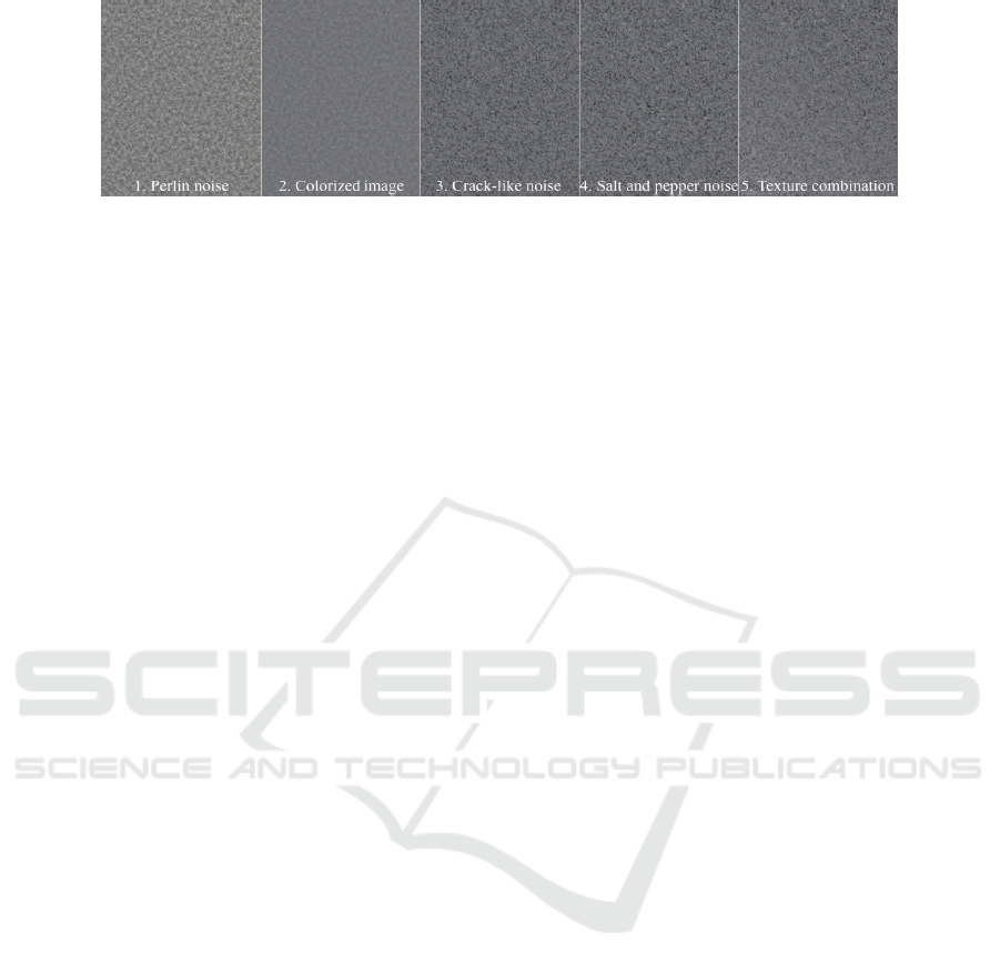
Figure 1: Illustration of the Syncrack’s background generation steps.
of these values are obtained based on user-provided
parameters, allowing user customization of the out-
put. To ensure reproducibility, the random value se-
lection is done with a fixed seed.
The user parameters relevant for our experiments
are described in this paper. For further information
about all the user parameters, as well as the random
value selection for internal parameters, we invite the
reader to visit our repository (provided at the end of
this article).
3.1 Background Generation
Our method (illustrated in Fig. 1) consists of 5 main
steps:
1. Creating a 2D Perlin Noise. By using the noise
module (Duncan, 2018), we create a noise map
based on Perlin noise (Perlin, 1985). The ‘scale’
parameter for the Perlin noise follows a normal
law defined by the background average smooth-
ness and standard deviation provided as user pa-
rameters to run the program.
2. Converting to color image. Public crack datasets
contain RGB images; even though the material
generally looks gray, the hue is not strictly zero.
To emulate the appearance of real materials, two
random, low saturated, colors are chosen to repre-
sent the darkest and the lightest regions in the Per-
lin noise. We merge these colors together with a
weighted average using the Perlin noise as weight.
3. Adding crack-like noise. Crack-like artifacts are
added to the image to make crack detection a chal-
lenge. To do this, we chose random pixels as cen-
ters to draw arcs of random size ellipses. Then,
we introduce these lines to the image similarly to
how cracks are introduced (see subsection 3.3).
The amount of noise is inversely correlated to the
background average smoothness parameter in 1.
4. Adding additional noise. Real images are prone to
invasive elements. We add salt and pepper noise
with different radii to simulate dirt on the surface
and acquisition artifacts. The amount of this noise
is inversely correlated to the background average
smoothness parameter too.
5. Combining different textures. Stationary textures
are not frequent in real-life constructions (spe-
cially in roads). We create non-stationary back-
ground by joining together two or more textures,
each one generated with steps 1-4. We combine
the textures with a linear gradient fill to create
smooth transitions.
3.2 Crack Shape Generation
Our crack shapes are based on a modification of the
1D Perlin noise. First, we calculate a set of ver-
tices using the Perlin noise generator from the noise
module. The domain of these vertices is determined
by a randomly chosen crack length -i.e. 0 ≤ x ≤
crackLength, ∀(x,y) ∈ vertices.
However, these vertices have two problems: 1)
their height scale (y-axis) is blind to the image size
and the crack length, and 2) they use a straight axis
as origin, so the cracks would always tend to straight
lines. To solve this, we normalize the y-coordinates
of the vertices to the range [0, 1] and map them to
the range [0, crackHeight] with a randomly chosen
height. To obtain curve cracks, we displace the y-
coordinates of the vertices using an elliptic function.
These vertices are connected with straight lines to
create a crack skeleton. To provide the crack with
width, we dilate the skeleton by a disk. The diam-
eter is chosen randomly from a normal distribution
centered at 2 with standard deviation 0.5 (default user
parameters). Since real cracks do not have constant
widths, a sliding-window approach is used to intro-
duce dilations and erosions in random crack regions.
To avoid drastic changes, the structuring element is
a 2-pixel long vertical line. Aditionally, a dilation is
never followed by an erosion or vice-versa. An exam-
ple of a final crack shape is shown in Fig. 2.
3.3 Crack Introduction
Once a crack shape is obtained, we generate a weight
map (same size as the background image) by creating
Syncrack: Improving Pavement and Concrete Crack Detection through Synthetic Data Generation
149

Figure 2: A synthetic crack shape generated by Syncrack.
an empty white image (weight=1.0) and putting a ran-
domly rotated version of the crack shape in a random
position within the new image (weight=0.0).
An average contrast value is randomly chosen
from a normal distribution with center and standard
deviation provided as user parameters. Then, within
the weight map, we set each crack-labeled pixel to
a new independent value. Per pixel, this value is
obtained from a new Gaussian distribution using the
chosen average contrast value as mean.
Since different crack regions tend to have different
lightning conditions in real life, we change the con-
trast of certain zones within the crack using a sliding
window. Finally, by using disk mean filters, we cre-
ate a transition region between the actual crack and
near-to-crack background. An example of the result-
ing weight map is shown in Fig. 3.
Figure 3: Example of a weight map used to introduce the
crack shape in Fig. 2 into a background image.
We use this weight map to introduce the crack into
the background by weighting each color channel with
the map. Fig. 4 shows an example of cracks inserted
in different backgrounds with different contrasts.
3.4 Label Noise Generator
To simulate inaccurate labeling, we introduce noise in
the annotations. We divide the annotation image into
tiles. Then, we alter randomly chosen tiles by per-
forming an erosion or a dilation by a disk with a ran-
dom diameter. With default user parameters, the tile
size is 0.05 ∗ imageHeight × 0.05 ∗ imageWidth. The
diameter of the the disk follows a normal law centered
around 3 for dilation and 2 for erosion. In both cases,
the standard deviation is 0.5.
The user parameter ‘noise percentage’ (np from
now on) is the probability, np ∈ (0, 1], for a tile to be
altered. Since the tiles are obtained by dividing the
whole image, and the probability is unconditional, an
altered tile may contain no cracks.
With np < 1, we expect inaccuracy similar to a
manual one: some crack segments wider (a dilation
was applied), some segments thinner (a small ero-
sion), missing crack segments (big erosion), and some
accurate segments. See Fig. 5 for examples.
4 EXPERIMENTAL SETUP
4.1 Evaluation Scores
We use two kind of evaluations: supervised and un-
supervised. The supervised scores compare the ob-
tained predictions and the available ground truth an-
notations. We used Precision (Pr) and Recall (Re), as
commonly done in the crack detection literature. The
harmonic mean of both yields a single metric – the F-
score. We used its equivalent, the Dice score, easily
allowing to add a smoothing factor to avoid division
by zero in images with no cracks (see last term of Eq.
4 below).
However, as discussed in this paper, when annota-
tions are inaccurate, supervised scores are biased. To
validate our results on real images, we propose a set
of metrics used previously for the evaluation of unsu-
pervised segmentation tasks (Zhang et al., 2008).
The first one is the crack region entropy H
crack
,
based on the region entropy (Pal and Bhandari, 1993).
Given the set R
c
of pixels within a crack-predicted re-
gion, define a set V
c
of all the possible pixel intensities
within R
c
. Define L
c
(m) as the amount of pixels with
intensity m ∈ V
c
within R
c
. Then
H
crack
(R
c
) = −
∑
m∈V
c
L
c
(m)
|R
c
|
log(
L
c
(m)
|R
c
|
) (1)
This is a way to measure the intra-crack uniformity.
Introducing background pixels into R
c
will increase
H
crack
(R
c
). A good crack prediction should reduce
the crack region entropy.
We also use a second-order crack region en-
tropy H
2
crack
. The second order-entropy relies on co-
occurrence matrices rather than pixel intensities. This
allows inspecting the intra-crack region for textures.
Given p the probability from the co-occurrence ma-
trix calculated in R
c
:
H
2
crack
(R
c
) = −
∑
i∈V
c
∑
j∈V
c
p
i j
log(p
i j
) (2)
Similarly to the first order entropy, including back-
ground pixels in R
c
will increase the entropy. A good
segmentation reduces this score.
We assume that cracks and background are two
different distributions. We use the Kolmogorov-
Smirnov test (Smirnov, 1939) to measure the distance
between the distributions of pixels predicted as crack
VISAPP 2022 - 17th International Conference on Computer Vision Theory and Applications
150
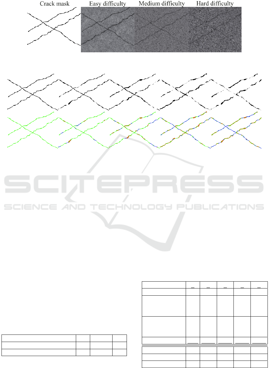
Figure 4: Syncrack images generated with different user parameters. The crack mask is the same, but the background
generation and crack-introduction parameter values differ to create different levels of difficulty for crack detection.
Figure 5: Examples of different label noise levels for Fig. 4. From left to right, levels 0 to 4 (see Table 2). The second row
shows: Green) Crack pixels; Blue) Crack pixels mislabeled as background; Red) Background pixels mislabeled as crack.
and as background, respectively. If both distribu-
tions differ, the Kolmogorov-Smirnov score (K-S) in-
creases. Therefore, we want to maximize this score.
All our metrics are calculated per image, and the
results shown in the rest of the paper are the averages
over all the analyzed images.
4.2 Synthetic Datasets
In this paper, we use 3 datasets (200 images each)
obtained with the Syncrack generator using different
user parameter values. Particularly, we modified 2
parameters: the background average smoothness (re-
ferred to as bas) and the crack average contrast (re-
ferred to as cac). The background smoothness in-
tervenes both in the Perlin noise generation and the
amount of added noise (see subsection 3.1). The crack
contrast modifies the relative contrast between the
background and the added crack (see subsection 3.1).
By modifying these two parameters, we create Syn-
crack datasets with 3 difficulty levels as described in
Table 1.
Table 1: Parameters used to create the 3 difficulty versions.
Difficulty level Easy Medium Hard
Background smoothness (bas) 6.0 3.0 1.5
Crack contrast (cac) 0.5 0.7 0.7
The easy difficulty has a smooth background and
well-contrasted cracks. The medium difficulty (de-
fault values) has rough textures with low-contrast
cracks. The hard example has the same contrast as
the medium one, but the background is rougher. The
3 datasets share the same cracks (see Fig. 4 for exam-
ple).
To study the effect of different label noise levels
in annotations used for training, we create noisy ver-
sions of the 3 above mentioned datasets. Particularly,
we introduce 5 label noise levels from 0 (no noise)
to 4 (the maximum amount of noise) by varying the
values of the np parameter (see subsection 3.4).
An analysis of the generated noise is pre-
sented in Table 2. The crack-to-background and
background-to-crack mislabeling percentages are cal-
Table 2: Label noise levels used for experiments.
Label noise level 0 1 2 3 4
np 0.00 0.25 0.50 0.75 1.00
Crack →
Background
mislabeling (%)
0.00 9.68 19.35 29.03 38.71
Background →
Crack
mislabeling (%)
0.00 12.90 24.19 32.26 43.55
Mislabeling (%) 0.00 22.58 43.55 61.29 82.26
DSC (%) 100 88.93 78.41 68.39 58.94
Pr (%) 100 88.44 77.18 68.53 58.29
Re (%) 100 89.92 80.61 69.41 60.66
Syncrack: Improving Pavement and Concrete Crack Detection through Synthetic Data Generation
151

Figure 6: U-VGG19’s architecture.
culated with respect to the total number of crack
pixels. For example, with 100 crack pixels in
the dataset: if 10 crack pixels were labeled as
background, Crack→Background mislabeling (%) =
10; if 5 background pixels were labeled as crack,
Background→Crack mislabeling (%) = 5. Mislabel-
ing (%) is the sum of both percentages. To understand
better the behavior of these percentages, we show the
DSC, precision and recall with respect to the clean
annotations too. Fig. 5 illustrates the different label
noise levels for Fig. 4.
4.3 Real Road Images
To validate the performance of models trained with
Syncrack on real-life data, we use the CrackForest
Dataset (CFD). This public dataset contains 118 im-
ages collected from urban roads containing perturba-
tions such as shadows, oil spots, and water stains in
Beijing, China (Shi et al., 2016). Similarly to the de-
fault size of the Syncrack generator, the original im-
age size is 480×320. The cracks in this dataset have a
width around 3 pixels, again similarly to the default
Syncrack generator. This dataset provides two an-
notations: borders and segmentation. As suggested
by (Sun et al., 2020), we removed some images with
clear severe annotation errors; we kept 108 images.
4.4 Baseline Model
U-net (Ronneberger et al., 2015), a symmetrical auto-
encoder, has seen success in pavement distress seg-
mentation. Similarly, VGG has been an attractive fea-
ture extractor to detect cracks (Escalona et al., 2019;
Zhang et al., 2020b). Based on this, we built a U-net-
like network using the pre-trained VGG19 (Simonyan
and Zisserman, 2015) as a basis.
This network, referred to as U-VGG19, is used as
a baseline model for our experiments (see Fig. 6).
4.5 Training Setup
We implemented the proposed architecture using Ten-
sorflow 2.1.0. For training, input images are cropped
to 256×256 patches and fed as 4-patch batches. We
used the Adam optimizer with a 10
−4
learning rate
and default parameters. The initial weights from
the encoder are the weights from VGG19 pre-trained
on ImageNet; from this starting point, the whole U-
VGG19 is trained together. Each dataset is randomly
split into 50% training and 50% validation.
Our preliminary models trained on synthetic im-
ages failed to detect cracks within color outlier pic-
tures. For example, bluish-looking pavement in con-
trast with the normal grayish colors. Since learning
models are sensitive to color information, we wish to
neglect the effect of color saturation due to the acqui-
sition process. To do this, all images are converted to
grayscale and converted back to 3 channels by con-
catenation.
To avoid overfitting to the distributions used by the
Syncrack generator, we trained using data augmenta-
tion. Our data augmentation consisted of randomly
transforming an image (and its corresponding annota-
tion) immediately before feeding it to the neural net-
work for training. To do this, a random value for
each of the 6 following operations is chosen: adding
noise, changing illumination, flipping, zooming, ro-
tating and shearing. Every image undergoes the 6 op-
erations in the given order.
To refine the results at late epochs, we reduce the
learning rate on validation loss plateau (by 2, with
5 epochs tolerance). To avoid overfitting, we add
an early stop if the validation loss does not decrease
during 20 consecutive epochs. We report the scores
calculated on the validation split using the network
weights with the minimum validation loss.
The loss is a combination of the binary cross-
entropy loss (BCE) and a DSC-based loss (DICE):
Loss = BCE + α ∗DICE (3)
Here, α is a hyperparameter (Sun et al., 2020) set em-
pirically to 3 to give more importance to DICE, cal-
culated as follows:
DICE = 1 −
2(GT · Pred) + 1
GT + Pred +1
(4)
Here, GT is the set of pixels annotated as crack and
Pred is the set of pixels predicted as crack. The more
similar GT and Pred are, the lower is DICE.
VISAPP 2022 - 17th International Conference on Computer Vision Theory and Applications
152
5 EFFECT OF DIFFERENT
NOISE CONDITIONS
To validate the unsupervised segmentation scores pro-
posed in this paper, we analyze their behavior under
controlled conditions. To do this, we use the noisy
annotations obtained with the Syncrack generator.
In this section, we first analyze the ability of un-
supervised scores to assess the quality of crack de-
tection using inaccurate annotations as reference. Af-
terwards, we use these inaccurate annotations to train
the baseline model (U-VGG19). Finally, we analyze
the relation between the unsupervised scores and the
prediction quality of trained models (one model per
noise and difficulty level).
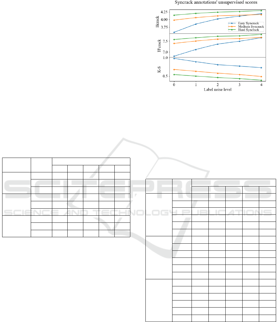
In Table 3, we summarize the unsupervised scores
calculated on the three difficulty versions of Syncrack
using the automatically generated annotations (with
different label noise levels).
Table 3: Unsupervised evaluation of the Syncrack generated
annotations.
Difficulty Metric
Label noise level
0 1 2 3 4
Easy
H
crack
3.58 3.85 4.02 4.11 4.19
H
2
crack
6.80 7.11 7.36 7.49 7.65
K-S 0.98 0.89 0.81 0.77 0.73
Medium
H
crack
3.98 4.06 4.12 4.14 4.16
H
2
crack
7.39 7.50 7.59 7.61 7.67
K-S 0.68 0.63 0.58 0.54 0.49
Hard
H
crack
4.14 4.20 4.24 4.26 4.29
H
2
crack
7.57 7.65 7.72 7.74 7.80
K-S 0.54 0.50 0.46 0.43 0.39
With 0 noise in the annotations, when the diffi-
culty level increases, both entropies increase too and
the K-S decreases (see Fig. 7). This is natural, since
it becomes harder to tell the difference between crack
and background by looking at the images.
More importantly, we observe a relation between
mislabeling and the unsupervised scores: as the anno-
tations become more inaccurate, the region entropies
increase and the K-S decreases. With this conclu-
sion, we extend our study using unsupervised scores
to evaluate predictions obtained with U-VGG19 (the
proposed baseline model for crack detection).
In this experiment, we trained U-VGG19 with the
different difficulty and label noise levels proposed for
Syncrack in this paper. In this way, we can observe 1)
the effect of training with noisy labels when evaluat-
ing with accurate annotations and 2) the relation be-
tween supervised and unsupervised scores when hav-
ing accurate labels for evaluation.
The results of this experiment are shown in Table
Figure 7: Unsupervised evaluation of the Syncrack gener-
ated annotations.
4. By analyzing the 0 noise column, we observe the
impact of the difficulty level in the prediction scores.
While the model on easy difficulty obtains supervised
scores above 96%, they decrease drastically as the
difficulty increases. Just as before, the unsupervised
scores get worse as we increase the difficulty level.
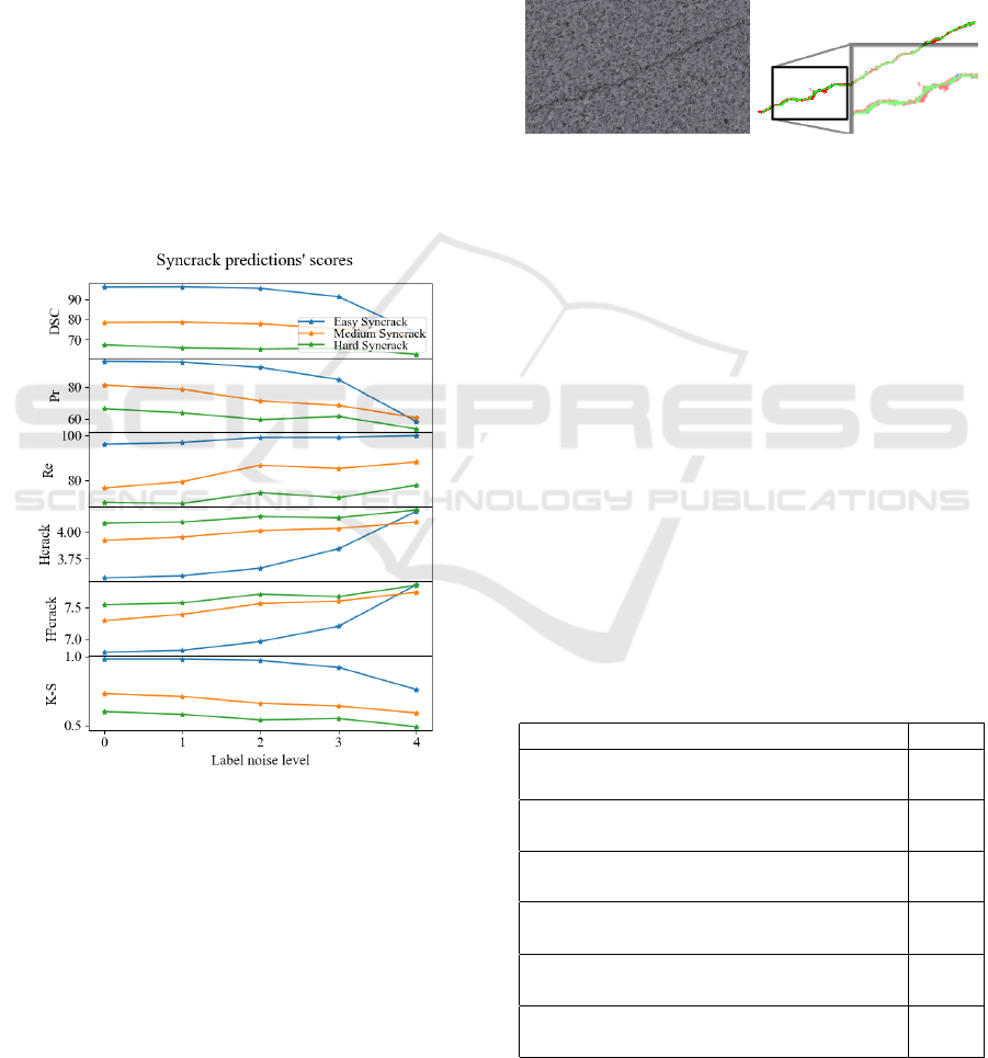
Table 4: Prediction scores obtained in the validation splits
of the Syncrack’s 3 difficulty levels.
Difficulty Metric
Label noise level
0 1 2 3 4
Easy
DSC 96.07 96.21 95.55 91.31 73.50
Pr 96.14 95.69 92.30 84.74 58.39
Re 96.03 96.77 99.07 99.09 99.80
H
crack
3.57 3.59 3.66 3.84 4.19
H
2
crack
6.79 6.82 6.96 7.20 7.86
K-S 0.98 0.98 0.97 0.92 0.76
Medium
DSC 78.43 78.58 77.86 75.49 71.45
Pr 81.17 78.58 71.30 68.44 60.75
Re 76.55 79.36 86.71 85.25 88.12
H
crack
3.92 3.95 4.01 4.03 4.09
H
2
crack
7.29 7.39 7.56 7.60 7.74
K-S 0.73 0.71 0.66 0.64 0.59
Hard
DSC 67.44 65.91 65.29 65.70 62.58
Pr 66.30 63.85 59.54 61.55 53.70
Re 70.17 69.67 74.47 72.21 77.81
H
crack
4.08 4.09 4.14 4.13 4.20
H
2
crack
7.54 7.57 7.71 7.67 7.85
K-S 0.60 0.58 0.54 0.55 0.49
However, it is important to compare the unsuper-
vised scores of the predictions with respect to the an-
notations. When 0 label noise is present, in the easy
difficulty, both the annotation and the prediction su-
pervised scores are very close; this is true as well for
the unsupervised scores. Nonetheless, for the other
difficulties, the unsupervised scores are slightly better
even though the supervised scores are lower.
Syncrack: Improving Pavement and Concrete Crack Detection through Synthetic Data Generation
153
This kind of behavior can be explained by two fac-
tors. 1) The severe class unbalance; if a few pixel
change in the crack region is numerically measurable
it may be not in the background region (which is by
far more populated). 2) As a consequence of the pre-
vious, the unsupervised scores are blind to false neg-
atives. Missing cracks won’t affect these scores. This
bias emphasizes the predictions when only pixels with
high likelihood of being crack pixels are segmented,
even at the cost of missing cracks or having isolated
false positives. Thus, these unsupervised scores must
be understood under this context and should be paired
with supporting supervised scores to be able to draw
conclusions.
With this in mind, we still observe that both the
supervised and unsupervised scores get worse as we
increase the label noise (see Fig. 8). This suggests
that the unsupervised scores can be used as indicators
of segmentation quality regardless of the annotation
quality.
Figure 8: Prediction scores obtained in the validation splits
of the Syncrack’s 3 difficulty levels evaluating with accurate
annotations.
It is interesting to notice that the DSC seems to in-
dicate noise robustness in the trained models: as we
increase the label noise level, the DSC of the predic-
tion (Table 4) tends to be higher than the DSC of the
annotations (Table 2).
However, this apparent robustness is a trade-off
between precision and recall. As the noise increases,
the recall tends to increase too; nonetheless, the pre-
cision decreases more. From this, we can hypothesize
that using noisy annotations may actually help to de-
tect harder cracks at the cost of having a considerable
amount of false positives. The presence of these false
positives is congruent with the behavior of the unsu-
pervised scores: both entropies increase while the K-
S decreases.
When we analyzed the predictions qualitatively,
the conclusion was that the main source of false posi-
tives was having crack predictions wider than the ac-
curate clean annotation (see Fig. 9).
Figure 9: Example of inaccurate prediction training with
label noise level 4. The color code is the same as in Fig. 5.
Taking this into account, when it comes to the
predicted cracks’ width, we observe a relation be-
tween precision and the proposed unsupervised met-
rics. With these preliminary results, we moved to real
road images for evaluation of our synthetic generator.
6 IMPROVING REAL-LIFE
CRACK DETECTION WITH
SYNCRACK
To have a baseline for real data, we trained U-VGG19
with our CFD training split. Table 5 compares our re-
sults with other methods based on deep learning when
no tolerance margins are used for evaluation. The
chosen metric was F-score, since it is the most com-
mon score used in the literature.
Table 5: F-scores on CFD without tolerance margins.
Method F-score
U-net
(Gao et al., 2019)
60.48%
GANs
(Gao et al., 2019)
64.13%
Multi-scale Convolutional Blocks
(Sun et al., 2020)
a
74.19%
Feature Pyramid and Hierarchical Boosting
(Yang et al., 2020)
b
70.50%
Distribution equalization learning
(Fang et al., 2021)
54.55%
U-VGG19
–(ours)–
70.27%
a
Training/Evaluation using a CFD+Aigle-RN dataset.
b
GT and Pred are thinned to 1-pixel edges for evaluation.
VISAPP 2022 - 17th International Conference on Computer Vision Theory and Applications
154
From this table, we confirm that U-VGG19 is a
competitive model with respect to the state of the art
when training with real-life data. Thus we use the
scores of this model as a baseline to compare with the
results obtained by training with Syncrack variants.
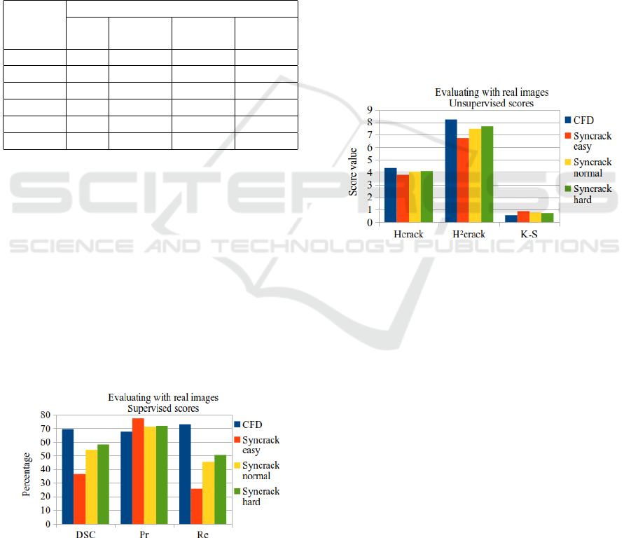
Table 6 shows the prediction scores of the mod-
els trained on CFD and on the 3 difficulty versions of
Syncrack. For these experiments, we trained on the
training split of each respective dataset and calculated
the scores on the CFD validation split. The models
trained on Syncrack were trained using accurate an-
notations.
Table 6: Scores obtained in the CFD validation set by using
models trained on different datasets.
Metric
Training dataset
CFD
Syncrack
easy
Syncrack
medium
Syncrack
hard
DSC (%) 69.32 36.37 54.26 58.26
Pr (%) 67.71 77.42 70.96 71.98
Re (%) 73.03 25.71 45.37 50.4
H
crack
4.35 3.79 4.07 4.12
H
2
crack
8.22 6.73 7.49 7.67
K-S 0.57 0.87 0.78 0.73
A plot of the supervised scores is shown in Fig.
10. We can see that the models trained with Syn-
crack datasets exhibit a higher precision than the
model trained on real images. However, we see a de-
crease of recall. Since the decrease in recall is higher
than the precision increase, the DSC of the models
trained with synthetic data are lower than the one of
the model trained with CFD. Particularly, the model
trained on the easy Syncrack has both the higher pre-
cision and the lower recall of all the datasets. As
we increase the Syncrack difficulty, the precision de-
creases a bit but the recall sees a great increase.
Specifically, the recall increases as we increase the
Syncrack difficulty level.
Figure 10: Supervised scores obtained in the CFD valida-
tion set by using models trained on different datasets.
Since the easy Syncrack has only easy-to-detect
cracks, a model trained with this dataset will strug-
gle to detect cracks with low contrast or rough back-
grounds. Thus, there is a high confidence in the pixels
predicted as cracks but the model will miss hard-to-
detect cracks. As we increase the Syncrack difficulty
level, the learned models will detect harder cracks (in-
creasing recall) but will incur in more false positives
(decreasing precision). The model trained with the
hard Syncrack has a better trade-off between preci-
sion and recall, obtaining a DSC of 58.26% in con-
trast with the 69.32% obtained by training with CFD.
This DSC difference is caused only by a decreased
recall. Assuming that manual annotations tend to be
wider than the actual cracks, a more precise segmen-
tation will lead indeed to a lower recall. Fig. 11 shows
the unsupervised scores from the models trained with
the different datasets. We can observe that the mod-
els trained with Syncrack have better scores than the
one trained on CFD. As we increase the Syncrack dif-
ficulty level, the entropies in the predicted crack re-
gions increase and the K-S decreases. Even for the
hard difficulty, these scores are better than for CFD.
Figure 11: Unsupervised scores obtained in the CFD vali-
dation set by using models trained on different datasets.
The hypothesis is that the decrease in recall is
caused mainly by missing some pixels in the exces-
sively wide annotations. A qualitative analysis of
the predictions confirmed this: as illustrated in Fig.
12, the performance of the models trained with the
medium and hard difficulty, respectively, get very
promising results. Not only they do a good job by not
missing cracks, but the predicted width looks more
close to the actual crack that both the annotation and
the prediction of CFD (see Fig. 13).
The model trained on medium Syncrack produces
refined segmentations but prone to contain small dis-
continuities. The model trained on hard Syncrack
tends to fill these gaps, but its predictions look more
coarse. However, using Syncrack generated images
showed their promising potential for supervised crack
detection without requiring labeled real-life images.
Syncrack: Improving Pavement and Concrete Crack Detection through Synthetic Data Generation
155
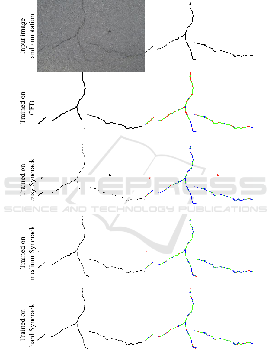
Figure 12: Example of predictions on a CFD image. The first row shows the input image and the provided annotation. The
next rows show the predictions of models trained on the different proposed datasets and its comparison with the manual
annotation (with the color code used in Fig. 5).
VISAPP 2022 - 17th International Conference on Computer Vision Theory and Applications
156
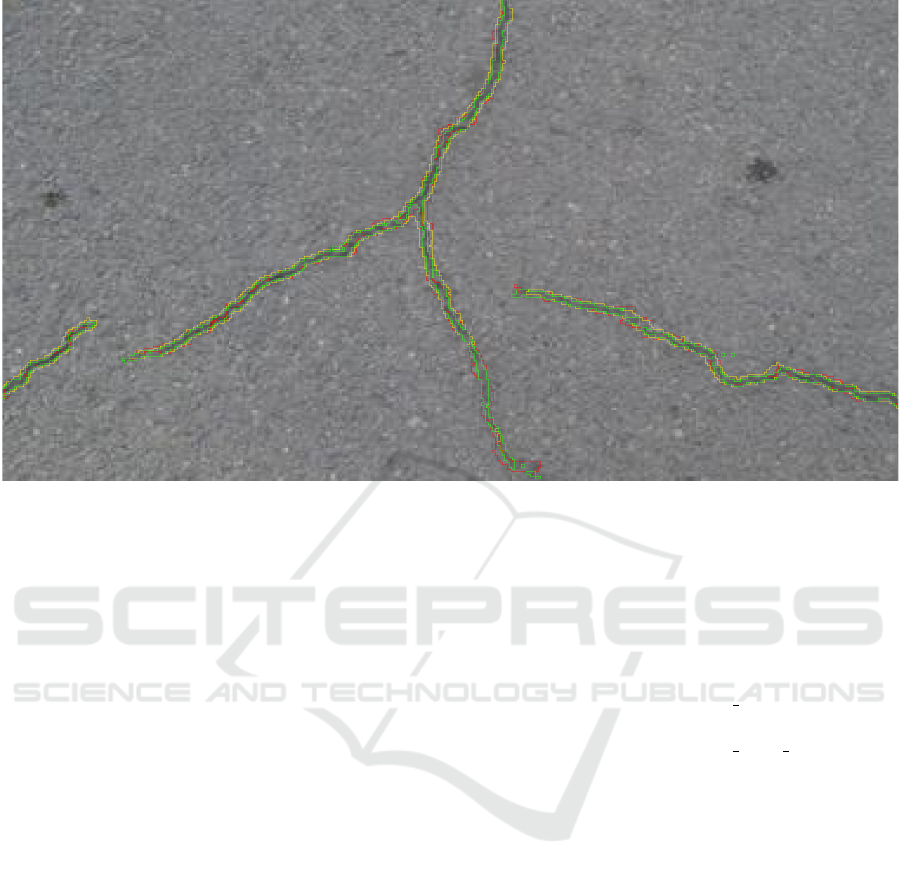
Figure 13: A close-up detailed view of the picture depicted in Fig. 12. The red line is the border of the manual annotation,
the yellow line is the border of the prediction obtained by training on CFD, and the green line is the border of the prediction
obtained by training on Syncrack hard.
7 CONCLUSIONS
In this paper, we introduced the Syncrack generator
–a tool aimed to create synthetic pavement/concrete
images with accurate annotations for crack detection.
By introducing mislabeling, this tool allows generat-
ing noisy versions of the labels to emulate the inaccu-
racy of manual annotations.
With both accurate and noisy labels, we studied
the impact of inaccurate annotations on supervised
segmentation scores as well as a set of proposed un-
supervised scores. These metrics (region entropies
and the Kolmogorov-Smirnov score) were used since
supervised scores are biased by human error in real
data. From these experiments, we found a relation
between the proposed scores and the prediction preci-
sion. However, further work is needed towards met-
rics that are blind to human annotations for this task.
Using these unsupervised scores as a basis, we
evaluated on real-life images the performance of mod-
els trained on Syncrack-generated datasets. Our re-
sults show competitive scores in terms of precision
with respect to real-data training. Although there is
an apparent decrease of recall, this behavior is due
mainly to the excessive width of manual annotations.
This is shown by the unsupervised scores as well as
the qualitative analysis.
Thus, the models trained solely with our syntheti-
cally generated data are competitive with the model
trained on real images; furthermore, they are more
precise in terms of crack width.
The Syncrack generator is available at: https://
github.com/Sutadasuto/syncrack
generator. The code
used to obtain our results is available at: https://
github.com/Sutadasuto/syncrack crack detection
ACKNOWLEDGEMENTS
This work has been supported by the project DiXite.
Initiated in 2018, DiXite (Digital Construction Site) is
a project of the I-SITE FUTURE, a French initiative
to answer the challenges of sustainable city.
REFERENCES
Ai, D., Jiang, G., Siew Kei, L., and Li, C. (2018). Au-
tomatic Pixel-Level Pavement Crack Detection Using
Information of Multi-Scale Neighborhoods. IEEE Ac-
cess, 6:24452–24463. Conference Name: IEEE Ac-
cess.
Amhaz, R., Chambon, S., Idier, J., and Baltazart, V. (2016).
Automatic Crack Detection on Two-Dimensional
Pavement Images: An Algorithm Based on Mini-
mal Path Selection. IEEE Transactions on Intelligent
Syncrack: Improving Pavement and Concrete Crack Detection through Synthetic Data Generation
157

Transportation Systems, 17(10):2718–2729. Confer-
ence Name: IEEE Transactions on Intelligent Trans-
portation Systems.
Bhat, S., Naik, S., Gaonkar, M., Sawant, P., Aswale, S., and
Shetgaonkar, P. (2020). A Survey On Road Crack De-
tection Techniques. In 2020 International Conference
on Emerging Trends in Information Technology and
Engineering (ic-ETITE), pages 1–6.
Coquelle, E., Gautier, J.-L., and Dokl
´
adal, P. (2012). Au-
tomatic assessment of a road surface condition. In
7th Symposium on Pavement Surface Characteristics,
Surf, Norfolk, Virginia.
Duncan, C. (2018). noise. https://github.com/caseman/
noise.
Escalona, U., Arce, F., Zamora, E., and Sossa Azuela, J. H.
(2019). Fully Convolutional Networks for Automatic
Pavement Crack Segmentation. Computaci
´
on y Sis-
temas, 23(2):451–460–460. Number: 2.
Fang, J., Qu, B., and Yuan, Y. (2021). Distribution equal-
ization learning mechanism for road crack detection.
Neurocomputing, 424:193–204.
Fr
´
enay, B. and Verleysen, M. (2013). Classification in the
presence of label noise: a survey. IEEE transactions
on neural networks and learning systems, 25(5):845–
869.
Gao, Z., Peng, B., Li, T., and Gou, C. (2019). Genera-
tive Adversarial Networks for Road Crack Image Seg-
mentation. In 2019 International Joint Conference on
Neural Networks (IJCNN), pages 1–8. ISSN: 2161-
4407.
Kanaeva, I. and Ivanova, J. A. (2021). Road pavement crack
detection using deep learning with synthetic data. In
IOP Conference Series: Materials Science and Engi-
neering, volume 1019, page 012036. IOP Publishing.
Kim, B. and Cho, S. (2018). Automated Vision-Based De-
tection of Cracks on Concrete Surfaces Using a Deep
Learning Technique. Sensors, 18(10):3452. Number:
10 Publisher: Multidisciplinary Digital Publishing In-
stitute.
Liu, Z., Cao, Y., Wang, Y., and Wang, W. (2019). Com-
puter vision-based concrete crack detection using U-
net fully convolutional networks. Automation in Con-
struction, 104:129–139.
Mazzini, D., Napoletano, P., Piccoli, F., and Schettini, R.
(2020). A Novel Approach to Data Augmentation for
Pavement Distress Segmentation. Computers in In-
dustry, 121:103225.
Oliveira, H. and Correia, P. L. (2014). CrackIT — An im-
age processing toolbox for crack detection and char-
acterization. In 2014 IEEE International Conference
on Image Processing (ICIP), pages 798–802. ISSN:
2381-8549.
Pal, N. R. and Bhandari, D. (1993). Image thresholding:
Some new techniques. Signal Processing, 33(2):139–
158.
Perlin, K. (1985). An image synthesizer. ACM Siggraph
Computer Graphics, 19(3):287–296.
Ronneberger, O., Fischer, P., and Brox, T. (2015). U-Net:
Convolutional Networks for Biomedical Image Seg-
mentation.
Shi, Y., Cui, L., Qi, Z., Meng, F., and Chen, Z. (2016). Au-
tomatic Road Crack Detection Using Random Struc-
tured Forests. IEEE Transactions on Intelligent Trans-
portation Systems, 17(12):3434–3445. Conference
Name: IEEE Transactions on Intelligent Transporta-
tion Systems.
Simonyan, K. and Zisserman, A. (2015). Very Deep Con-
volutional Networks for Large-Scale Image Recogni-
tion. arXiv:1409.1556 [cs]. arXiv: 1409.1556.
Smirnov, N. V. (1939). On the estimation of the discrepancy
between empirical curves of distribution for two inde-
pendent samples. Bull. Math. Univ. Moscou, 2(2):3–
14.
Sun, M., Guo, R., Zhu, J., and Fan, W. (2020). Road-
way Crack Segmentation Based on an Encoder-
decoder Deep Network with Multi-scale Convolu-
tional Blocks. In 2020 10th Annual Computing and
Communication Workshop and Conference (CCWC),
pages 0869–0874.
Yang, F., Zhang, L., Yu, S., Prokhorov, D., Mei, X., and
Ling, H. (2020). Feature Pyramid and Hierarchi-
cal Boosting Network for Pavement Crack Detection.
IEEE Transactions on Intelligent Transportation Sys-
tems, 21(4):1525–1535. Conference Name: IEEE
Transactions on Intelligent Transportation Systems.
Yang, X., Li, H., Yu, Y., Luo, X., Huang, T., and
Yang, X. (2018). Automatic Pixel-Level Crack De-
tection and Measurement Using Fully Convolutional
Network. Computer-Aided Civil and Infrastruc-
ture Engineering, 33(12):1090–1109. https://online
library.wiley.com/doi/pdf/10.1111/mice.12412.
Zhang, H., Fritts, J. E., and Goldman, S. A. (2008). Image
segmentation evaluation: A survey of unsupervised
methods. Computer Vision and Image Understanding,
110(2):260–280.
Zhang, K., Zhang, Y., and Cheng, H.-D. (2020a). Crack-
GAN: Pavement Crack Detection Using Partially Ac-
curate Ground Truths Based on Generative Adversar-
ial Learning. IEEE Transactions on Intelligent Trans-
portation Systems, pages 1–14. Conference Name:
IEEE Transactions on Intelligent Transportation Sys-
tems.
Zhang, L., Shen, J., and Zhu, B. (2020b). A research
on an improved Unet-based concrete crack detec-
tion algorithm. Structural Health Monitoring, page
1475921720940068. Publisher: SAGE Publications.
Zhang, L., Yang, F., Daniel Zhang, Y., and Zhu, Y. J. (2016).
Road crack detection using deep convolutional neural
network. In 2016 IEEE International Conference on
Image Processing (ICIP), pages 3708–3712. ISSN:
2381-8549.
Zhou, Z.-H. (2017). A brief introduction to weakly super-
vised learning. National Science Review, 5(1):44–53.
Zou, Q., Cao, Y., Li, Q., Mao, Q., and Wang, S. (2012).
CrackTree: Automatic crack detection from pavement
images. Pattern Recognition Letters, 33(3):227–238.
VISAPP 2022 - 17th International Conference on Computer Vision Theory and Applications
158
