
Analysis of Computational Efficiency in Iterative
Order Batching Optimization
Johan Oxenstierna
1,2 a
, Jacek Malec
1b
and Volker Krueger
1c
1
Dept. of Computer Science, Lund University, Lund, Sweden
2
Kairos Logic AB, Lund, Sweden
Keywords: Order Picking, Order Batching Problem, Computational Efficiency, Warehousing.
Abstract: Order Picking in warehouses is often optimized through a method known as Order Batching, wherein several
orders can be assigned to be picked by the same vehicle. Although there exists a rich body of research on
Order Batching optimization, one area which demands more attention is that of computational efficiency,
especially for warehouses with unconventional layouts and vehicle capacity configurations. Due to the NP-
hard nature of Order Batching, computational cost for optimally solving large instances is often prohibitive.
In this paper we focus on approximate optimization and study the rate of improvement over a baseline solution
until a timeout, using the Single Batch Iterated (SBI) algorithm. Modifications to the algorithm, trading
computational efficiency against increased memory usage, are tested and discussed. Existing and newly
generated benchmark datasets are used to evaluate the algorithm on various scenarios. On smaller instances
we corroborate previous findings that results within a few percentage points of optimality are obtainable at
minimal CPU-time. For larger instances we find that solution improvement continues throughout the allotted
time but at a rate which is difficult to justify in many operational scenarios. The relevance of the results within
Industry 4.0 era warehouse operations is discussed.
1 INTRODUCTION
Order Picking is the process in which human pickers
or vehicles (henceforth vehicles) retrieve sets of
products (orders) from locations in a warehouse.
Order Batching is a method in which vehicles can be
assigned to pick several orders at a time. Order
Batching can be formulated as an optimization
problem known as the Order Batching Problem
(OBP) (Gademann et al., 2001) or the Joint Order
Batching and Picker Router Problem (JOBPRP)
(Valle et al., 2017), where the Picker Router Problem
is a Traveling Salesman Problem (TSP) applied in a
warehouse environment (Ratliff & Rosenthal, 1983).
We consider the OBP and JOBPRP versions
equivalent if solutions to the OBP are assumed to
include TSP solutions (henceforth we use the term
OBP to refer to this version). There are several further
versions and focus areas in OBP’s, including
dynamicity, traffic congestion, depot setups and
a
https://orcid.org/0000−0002−6608−9621
b
https://orcid.org/0000−0002−2121−1937
c
https://orcid.org/0000−0002−8836−8816
obstacle layouts. One area in need of more attention
is computational efficiency. As will be laid out in
Section 2, computational efficiency is considered
important in OBP-related research, but detailed
discussions are sparse and there are significant
differences in how CPU-times and timeouts are used.
Although the variability of OBP’s and results
concerning computational efficiency is high, we
believe more research in this domain is warranted.
We delimit our work to OBP’s where the aim is to
minimize aggregate distances, and as measurement of
computational efficiency we use the rate with which
aggregate distance is reduced through CPU-time over
a baseline solution. We use a distance based OBP cost
because this is the predominant Key Performance
Indicator (KPI) in OBP benchmark datasets.
Although a KPI based on capital cost is what is
mostly sought by warehouse management, it is
difficult to work with: There are a multitude of
complex and variable features that go into capital,
Oxenstierna, J., Malec, J. and Krueger, V.
Analysis of Computational Efficiency in Iterative Order Batching Optimization.
DOI: 10.5220/0010837700003117
In Proceedings of the 11th International Conference on Operations Research and Enterprise Systems (ICORES 2022), pages 345-353
ISBN: 978-989-758-548-7; ISSN: 2184-4372
Copyright
c
2022 by SCITEPRESS – Science and Technology Publications, Lda. All rights reserved
345
such as time-based aspects of work, traffic
congestion, maintenance, ergonomics etc. A distance
based KPI makes it easier to generate instances and
solutions in a more generalizable and reproducible
way.
For experimentation we use the approximate
optimizer Single Batch Iterated (SBI), to which we
introduce novel search heuristics that permit stronger
solution improvement at the cost of increased
memory usage. We only work with CPU-times in the
range 0 – 300 seconds. Results are compared with
previous work by Aerts et al. (2021) and Henn &
Wäscher (2012b), who have proposed approximate
optimization results for sets of smaller instance sizes.
For smaller instances we also assess SBI against
optimal results on the Foodmart dataset (Briant et al.
2020). For larger instances we introduce a new
dataset and make it available on a public repository
(Section 5.1). For instance generation we use the
TSPLIB format (Hahsler & Kurt, 2007). As far as we
are aware, there exists no standard benchmark format
in OBP research, rendering experiments difficult to
reproduce. Further discussions on how to represent
key OBP features in reproducible data is highly
relevant. This would allow for more data-driven
evaluation of algorithmic performance, for example
when investigating computational efficiency. Our
research aims are as follows:
1. To investigate the importance of
computational efficiency in OBP
optimization.
2. To analyse computational efficiency of an
approximate OBP optimizer on both existing
and new test-instances and to discuss results
in the light of previous work.
2 LITERATURE REVIEW
In this section we first present how the OBP and some
of its key features are formulated in the literature.
Then we present commonly used OBP optimization
algorithms and heuristics. Finally, we present how
computational efficiency has been motivated and
evaluated in different OBP scenarios.
As several studies have pointed out, the Order
Batching Problem (OBP) shares significant
similarities with the more well-known Vehicle
Routing Problem (VRP) (Cordeau et al., 2007; Valle
et al., 2017; Valle & Beasley, 2019). Aerts et al.
(2021), distinguish three points of separation between
the OBP and the standard VRP:
1. Order-integrity constraint: In the OBP the
products belonging to an order may only be picked by
one vehicle, whereas there exists no concept of orders
or order-integrity in the standard VRP.
2. Number of visits constraint: In the OBP the
same location may be visited several times by various
vehicles, whereas a location may only be visited once
in the standard VRP.
3. Obstacle-layout: In the OBP it is assumed that
there exists an obstacle layout, whereas there is no
such assumption in the standard VRP.
Concerning the latter point, most of the research on
the OBP assumes that the warehouse uses a
conventional layout, which means racks are arranged
with parallel aisles (between racks) and parallel cross-
aisles (between sections of racks). If these conditions
are not met the layout is unconventional (see Figure 1).
Aerts et al. argue that the OBP can be modelled as
a Clustered VRP (CluVRP) with weak cluster
constraints. Weak cluster constraints mean that a
vehicle may visit the locations in several clusters of
locations in any sequence. The CluVRP was first
introduced by Defryn & Sörensen (2017) and is
according to Aerts et al. equivalent to the OBP since
clusters can be mapped as orders. In experiments they
utilize this problem on a conventional layout
warehouse and on OBP scenarios involving up to 100
orders.
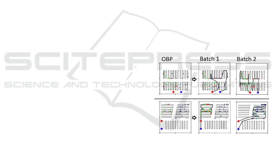
Figure 1: Examples of a conventional (top) and
unconventional (bottom) layout warehouse, and example
OBP’s with four orders. The colored diamonds denote
origin and destination locations. The colored dots denote
products and the orders which they belong to. In the
solutions (right of the arrows), one vehicle is assigned to
pick the red and lime orders and a second vehicle is
assigned to pick the blue and green orders.
For conventional layouts, proposed optimization
algorithms include integer programming (Valle et al.,
2017), clustering (Kulak et al., 2012), datamining
(Chen & Wu, 2005), dynamic programming (Briant
et al., 2020) meta-heuristics and heuristics: Examples
of meta-heuristics include Variable Neighborhood
Search (Aerts et al., 2021), Tabu Search (Henn &
Wäscher, 2012b), Ant Colony Optimization (Li et al.,
ICORES 2022 - 11th International Conference on Operations Research and Enterprise Systems
346

2017) and Genetic Algorithms (Cergibozan & Tasan,
2020). The heuristic algorithms can be divided into
three categories: Priority rule-based algorithms,
savings algorithms and seed algorithms (Henn et al.,
2010). Priority-rule based algorithms build batches by
sorting orders according to a heuristic, for example
First-Come-First-Serve, First-Fit or Best-Fit. In
savings algorithms batches with single orders are first
initialized and evaluated. Then, pairs, triplets and
larger collection of orders are constructed and the
combination with the best total result is retrieved
(Henn & Wäscher, 2012a). In seed algorithms batches
are generated in two phases: Seed selection and order
addition. In seed selection, an initial seed order is
chosen and then orders are added to the seed. There
are several proposals for how to choose the first seed
and add orders to it (Ho et al., 2008). One example is
the Sequential Minimal Distance (SMD) heuristic
(Sharp & Gibson, 1992), where the sum of minimal
distances between products in the seed order and
remaining orders is computed:
𝑆𝑀𝐷
𝑠,𝑜
𝑚𝑖𝑛
∈
𝑑
,
∈
𝑜∈𝒪,𝑜∉𝑏,𝑠∈𝑏,
(1)
where 𝑠 denotes a seed order in batch 𝑏, where 𝑜
denotes an order which does not exist in 𝑏, and where
𝑖 and 𝑗 denote products in order 𝑠 and 𝑜 respectively.
Whenever there are more than two products in a
batch, we assume some form of TSP algorithm is used
within the OBP algorithm. For conventional layouts,
the highly efficient S-shape or Largest Gap
algorithms are commonly used (Henn, 2012;
Roodbergen & Koster, 2001). We are not aware of
any attempts to extend these to unconventional
layouts. Given a distance matrix is provided,
however, TSP’s can be optimized reasonably fast
using e.g. OR-tools (Kruk, 2018) or Concorde (D.
Applegate et al., 2002; D. L. Applegate et al., 2006).
Computational efficiency in OBP optimization
can be motivated in two general ways. The first
concerns the direct impact of CPU-time on warehouse
operations. In models where orders are coming in to
the warehouse dynamically, for example,
optimization should ideally be faster than the time it
takes a vehicle to finish a picking round (Henn, 2012;
Scholz et al., 2017). Otherwise, vehicles must wait in
an idle state at the depot. Dynamic models are
generally more realistic than static ones (incoming
orders are there assumed to be known beforehand).
The literature still tends to model OBP’s as static
since dynamicity incurs more complexity (Scholz et
al., 2017).
The second motivation for computational
efficiency stems from a system architecture
perspective and how an OBP optimization module
can integrate with a Warehouse Management System
(WMS) without leading to higher optimization costs
in a more indirect sense. As an example, if an OBP
module is deployed on the cloud as a 3
rd
party
software service (SaaS) there are some advantages
with short CPU-times: A WMS client may be more
interested in buying a service if it is safe and simple
to integrate and this is made easier with short CPU-
times (Esposito et al., 2016). Furthermore, rental cost
of servers can be assumed to rise with CPU-time and
this also motivates more efficiency in regard to CPU-
times (Naumenko & Petrenko, 2021).
The efficiency considerations described above are
rarely considered of central importance in the broader
literature on the OBP, however. CPU times are
chosen to be “tolerable” (Kulak et al., 2012),
“reasonable” (Bozer & Kile, 2008), “acceptable” or
“realistic” (Aerts et al., 2021), but often lack in
explanations of what these terms actually entail.
Some examples are provided below for how
researchers have used CPU-times and timeouts in
optimization experiments with OBP’s.
For approximate optimization, Henn & Wäsher
(Henn & Wäscher, 2012a) use timeouts between 1 –
180 seconds for a heuristic optimizer and OBP’s
where 40 – 100 unassigned orders are to be batched.
Aerts et al. (2021), set timeouts between 1 and 60
seconds on the same instance set and propose a meta-
heuristic algorithm specifically designed to terminate
at around 60 seconds, since solution improvement is
found to be insignificant beyond that point. Both
Aerts et al. and Henn & Wäscher’s algorithms come
to within 5% of the best solution overall within the
first 10% of optimization time. Scholz et al. (2017)
experiment with instances of similar size but in a
dynamic setting and report a much lower efficiency:
70% of maximum allowed CPU-time is necessary to
reach within 5% of best solution overall. Efficiency
also decreases non-linearly with instance size in their
results: For 10 orders their optimizer needs 2 seconds,
for 100 orders it needs 11 minutes, and for 200 orders
60 minutes. Henn (2012) also presents an algorithm
for dynamic OBP’s and sets it to self-terminate after
60 seconds, partly due to operational considerations
(to avoid vehicles from idling at the depot). Many
publications do not present concrete results for
timeouts or rate of solution improvement, or a low
number of experiments (Azadnia et al., 2013; Bué et
al., 2019; Jiang et al., 2018). Kulak et al. (2012) and
Li et al. (2017), for example, present highly efficient
meta-heuristic optimizers, but use only 5 to 10
instances and do not show their rate of solution
improvement. For authors presenting algorithms
Analysis of Computational Efficiency in Iterative Order Batching Optimization
347

capable of finding optimal solutions to static OBP’s,
Henn & Wäscher (2012b), set timeouts between 2 –
1328 seconds for instances with up to 60 orders.
Gademann et al. (2001), set timeouts to 10 – 30
minutes for up to 100 orders. Valle et al. (2017) and
Briant et al. (2020), on the Foodmart dataset, present
timeouts in the range 300 seconds to 2 hours for 20-
30 orders.
These examples show that computational
efficiency in OBP experiments is difficult to judge
generally. Choice of static or dynamic modelling,
optimal versus approximative optimization,
experimental setup, instance sizes and the technology
level of used software and hardware, are all factors
that can have a complex effect on results in this
regard.
3 PROBLEM FORMULATION
We define the OBP objective as the assignment of
batches to vehicles such that the aggregate distance
needed to pick the batches is minimized. Each batch
𝑏 consists of a set of orders 𝑏∈2
𝒪
,𝑏∅ where
each 𝑜∈𝒪 is a subset of products 𝑜∈2
𝒫
,𝑜∅.
Each product 𝑝∈𝒫 is a set which includes a unique
product identifier, an order identifier, weight 𝑤 and
volume 𝑣𝑜𝑙, 𝑤,𝑣𝑜𝑙∈ ℝ
. The sum of weight,
volume or number of orders in a batch can be
retrieved with function 𝑞
𝑏
,𝑞∈𝑤,𝑣𝑜𝑙,𝑘. The x,
y location coordinates of all products is defined as set
ℒ
𝒫
, and the location of a product is retrievable with
function 𝑙𝑝. The locations of the products in an
order are retrievable with function 𝑙
𝑜
∪
∈
𝑙
𝑝
,
and all locations in a batch are retrievable with
function 𝑙
𝑏
∪
∈
𝑙
𝑜
. We define a single origin
location for all vehicles 𝑙
, a single destination
location 𝑙
and a set of polygonal obstacle location
sets ℒ
𝒰
. The aggregate of all locations is ℒ𝑙
∪
𝑙
∪ℒ
𝒫
∪ℒ
𝒰
.
We build undirected graph 𝐺𝑉,𝐸. Each
vertex in 𝑉 represents a unique location in ℒ and
function 𝑣
𝑙
gives a vertex for a location and 𝑙
𝑣
gives a location for a vertex. The vertices in batch 𝑏
includes the origin and destination vertices 𝑣
𝑏
𝑣
𝑙
∪𝑣𝑙
𝑏
∪𝑣
𝑙
. 𝐸 represents the set of all
Euclidean edges between all locations that
circumvent obstacles in ℒ
𝒰
. Distance matrix 𝐷 and
shortest paths between all edges is computed using
the Floyd-Warshall algorithm. How 𝐸 and shortest
paths can be constructed with polygonal obstacles is
beyond the scope of this paper; for details see
(Rensburg, 2019). We also permit several products to
be assigned to the same location in our model. This
can be useful to help reduce the memory footprint of
𝐺. The path to pick batch 𝑏 is retrievable with the
following function:
𝑇
𝑏
𝑣
,𝑛
|
𝑣
𝑏
|
,
(2)
𝑣
𝑣
𝑖1
𝑣
1𝑖𝑛
𝑣
𝑖𝑛
(3)
and represents the solution to a Traveling
Salesman Problem (TSP). The distance of 𝑇𝑏 is
retrievable with function
𝐷
𝑏
∑
𝑑
,𝑖,𝑗∈
ℤ
,𝑗𝑖1,𝑖
|
𝑇𝑏
|
, where 𝑑 represents entries
in distance matrix 𝐷. Vehicles are defined as 𝑚∈ℳ
where each vehicle has capacities expressed in weight
𝑤, volume 𝑣𝑜𝑙 and number of orders 𝑘. The scenario
where a vehicle 𝑚 is assigned a batch, order, and/or
product location is defined with binary variables 𝑥
,
𝑥
and 𝑥
, respectively. We then formulate the
OBP as follows:
𝑚𝑖𝑛𝐷
𝑏
𝑥
,
∈ℬ
𝑚∈ℳ
s.t.
(4)
𝑥
∈
ℳ
1,∀𝑜∈𝒪
(5)
𝑥
∈
𝑥
,∀𝑜∈𝒪,𝑚∈ℳ
(6)
𝑞
𝑏
𝑞
𝑚
𝑥
,𝑏∈ℬ,
𝑞∈𝑤,𝑣𝑜𝑙,𝑘,𝑚∈ℳ
(7)
where (4) states the objective, i.e., minimize
distances for all generated batches ℬ , where (5)
enforces order-integrity, where (6) enforces all
locations in all orders to be visited at least once and
where (7) ensures vehicle capacities are never
exceeded. Since this OBP is highly intractable we
also formulate a less ambitious objective in the single
batch OBP:
𝑎𝑟𝑔𝑚𝑖𝑛
∈ℬ
𝐷
𝑏
(8)
Here the aim is to find a single batch for an already
selected vehicle. For this case we also enforce the
single batch to come as close as possible to vehicle
capacity: ∃𝑞𝑞
𝑏
𝑞
𝑜
𝑞
𝑚
,∀𝑜∈𝒪,𝑜∉
𝑏,𝑞∈𝑤,𝑣𝑜𝑙,𝑘.
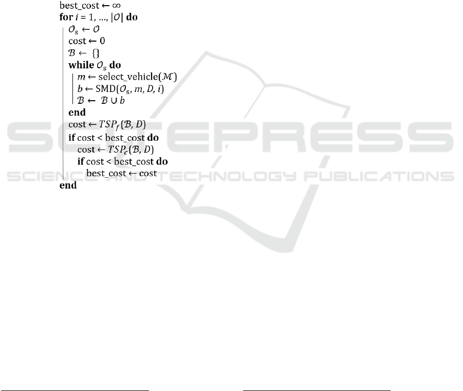
4 OPTIMIZATION ALGORITHM
SingleBatchIterated (SBI) (Algorithm 1) is a heuristic
multi-phase optimizer. In the core of the algorithm
ICORES 2022 - 11th International Conference on Operations Research and Enterprise Systems
348
unassigned orders 𝒪 are iteratively sent as input to the
SMD (Sequential Minimal Distance) seed function,
together with distance matrix 𝐷, a randomly chosen
available vehicle and a variable seed index. The SMD
function builds a single batch 𝑏 by first selecting a
seed order according to the seed index and adding
orders to it according to minimal distances (Equation
1). Batch 𝑏 is then removed from the set of
unassigned orders and the procedure repeats until all
orders have been batched into ℬ. An approximate
solution to the OBP can thus be obtained by pre-
selecting vehicles and approximately solving a single
batch OBP for that vehicle (Equation 8).
Algorithm 1: Single Batch Iterated (SBI).
The path to visit all locations in batch 𝑏∈ℬ, 𝑇
𝑏
and its distance, 𝐷
𝑏
, is computed using the OR-
tools TSP optimization suite
4
, in function TSP
f
. OR-
tools is set to finish quickly by using a number of
iterations parameter, which is set to grow linearly
with number of vertices in the TSP. If the aggregate
distance was found to be lower than the best result so
far, the TSP’s are optimally solved using Concorde
5
.
If the aggregate distance is still lowest, the solution is
stored as the best result.
The algorithm self-terminates after |𝒪| outer
loops (or after a manually set timeout of 300 seconds
in our experiments). Since the number of calls to
SMD is approximately cubic to number of orders:
|
𝒪
|∑|
𝒪
|
𝑖
,𝑖∈
|𝒪| 1
, we use an SMD order-
4
https://developers.google.com/optimization/routing/tsp,
collected 13-09-2021.
5
http://www.math.uwaterloo.ca/tsp/concorde/index.html,
collected 16-09-2021.
6
https://pagesperso.g-scop.grenoble inp.fr/~cambazah/
batching/, collected 04-05-2021.
order enumerated matrix, which is populated through
the optimization procedure: If SMD between two
orders does not exist in the matrix, it is computed and
pushed to the matrix. Once the value is stored it is
subsequently queried. Caching SMD’s this way
reduces number of calls to SMD from cubic to square,
at an insignificant increase of memory usage (~25
megabytes for 5000 orders assuming 8 bits per cell in
the matrix). It should be noted that this only works for
an SMD algorithm where the seed is defined as a
single order, which cannot provide more than a noisy
estimate of the subsequent TSP solution distance for
batches with more than two orders. We still deem
pairwise order-order SMD caching is suitable, since
distance estimates are inaccurate even if SMD’s for
larger collections of orders are computed (TSP
optimization is required for accurate estimates).
Caching could also be used to store all generated
single batches and their solved TSP’s in a hash tree or
equivalent, to prevent the same TSP to be optimized
twice (memoization). We leave an implementation of
this for future work, but there are likely gains to be
made in general by storing and reusing results from
the most expensive parts of the algorithm.
5 EXPERIMENTS
5.1 Benchmark Datasets
The publicly shared datasets Foodmart
6
, L6_203
7
and
L09_251
8
are used for experimentation. Foodmart
was introduced by Valle et al. (2017) and models a
warehouse with a conventional layout with a
maximum of 8 aisles and 3 cross-aisles. A feature in
Foodmart is that vehicles carry bins and that vehicle
capacity is expressed as a volume unit per bin. If an
order cannot fit in a single bin, splitting it between
different bins is permitted. SBI is not specifically
designed to optimize for this feature (an extra bin
packing problem within the OBP), so a greedy
heuristic module is appended to the optimizer for the
Foodmart experiment (for details see Oxenstierna et
al., 2021).
L6_203 and L09_251 model scenarios for up to
six unconventional warehouse layouts and multiple
depots. In these instances, vehicle capacity is
7
https://github.com/johanoxenstierna/OBP_instances, co-
llected 23-09-2021.
8
https://github.com/johanoxenstierna/L09_251, collected
10-06-2021.
Analysis of Computational Efficiency in Iterative Order Batching Optimization
349
expressed in number of orders. To allow for some
degree of comparability between L6_203 and
Foodmart, we chose to exclude the largest six
instances in Foodmart (100 – 5000 orders). Apart
from these the number of orders is similar between
Foodmart and L6_203. For larger instances we
instead use L09_251, where number of orders range
between 50 – 1000.
Number of orders only gives a rough idea of how
much CPU-time might reasonably be needed to
optimize an OBP instance. Number of products and
vehicle capacities are further examples of features
that have a considerable impact. To classify instances
by size, we use the amount of computational time SBI
requires to obtain a baseline solution: 0-2, 2-5, 5-7 or
7-10 seconds. The resulting number of instances for
the four classes are as follows: 0-2 s: 395, 2-5 s: 191,
5-7 s: 88, 7-10 s: 32. For all our experiments we use
Intel Core i7-4710MQ 2.5 GZ 4 cores, 16 GB RAM.
5.2 Experiment Results
Aggregations of all results are presented in Table 1,
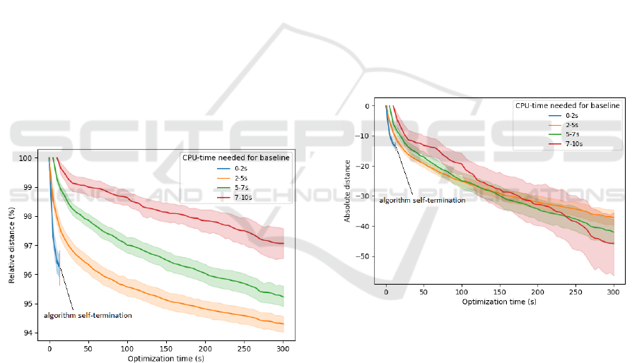
Figure 2 and Figure 3. In Figure 2, the average
improvement rate from the baseline is shown for the
four instance size classes. The shades around the lines
represent 95% confidence intervals.
Figure 2: Optimization time versus relative OBP distances
in percentages, for four instance size classes.
The solution improvement rates for smaller instances
(blue and orange) generally corroborate those of
Henn & Wäscher (2012b) and Aerts et al. (2021):
Improvements are significant in the initial stage of
optimization (1-4% improvement over baseline
within the first 10% of optimization) and then taper
off. In our case all instances with up to 100 orders
require no more than 2 seconds to obtain a baseline.
Within this class we also note SBI always self-
terminates within 10 seconds (in figures 2 and 3 we
show this by cutting the blue curve at 10 seconds; it
could also have been extended as a horizontal line
beyond 10 seconds).
The Foodmart instances fit within the smallest
class and there we compare against optimal results in
Briant et al. (2020): On average, a gap to optimality
of 2.3% was achieved after a maximum of 10
seconds. The gap between the baseline solution and
the best solution found was 3.2% on Foodmart. On
generated instances in L6_203 the corresponding gap
was 3.5%.
For our larger instance classes (2-10 seconds to
find a baseline solution), the pattern is similar, but
more time is needed to reach the same percentage
improvement over the baseline. This is expected since
fewer candidate solutions can be generated for larger
instances within the same CPU-time (more
computational time is needed by the SMD and TSP
functions to generate a solution).
In terms of absolute distance rate of improvement,
we first standardize the data such that the average
pick round is of similar length between the three
datasets. The absolute distance improvements for the
four instance size classes are shown in Figure 3:
Figure 3: Optimization time versus standardized absolute
distance savings, for four instance size classes.
Only toward the end of the maximum allotted CPU-
time we observe larger absolute gains for larger
OBP’s. As solution space grows, the probability of
SBI finding a strong baseline decreases and possible
improvement percentages can therefore be assumed
to be higher for larger instances. As we can see in
Figure 3, the red curve, for example, starts with the
least amount of distance saved compared to the other
curves, but ends with the most amount of distance
saved. The time to get there is 4 minutes, however.
This is explainable since larger instances require
more time to produce candidate solutions. Since there
are only 32 instances in the class of largest instances,
ICORES 2022 - 11th International Conference on Operations Research and Enterprise Systems
350

more data would be needed to investigate this pattern
further and to narrow the confidence intervals. The
less regular pattern and larger confidence interval in
the red curve is primarily assumed to be due to the
fewer number of data points.
Concerning rate of solution improvement, we can
see that it decreases to less than ~1% / minute after
the initial gains taper off after 30 – 60 seconds (Figure
2). In terms of standardized distance, this is on
average equivalent to around 18% of the length of a
single batch TSP solution (~12 standardized distance
units).
As discussed in Section 2, generalization of results
is difficult due to the high variability of OBP
scenarios. Overall, we believe 1% / min is a slow rate
of improvement and that it would be difficult to
justify in many scenarios, especially when
considering various indirect advantages of short
CPU-times (Section 2).
6 CONCLUSION
We investigated computational efficiency in
approximate Order Batching Problem (OBP)
optimization, both in previous work and in an
experiment involving the Single Batch Iterated (SBI)
optimizer. In previous work, computational
efficiency is rarely discussed in detail, especially for
warehouses with various types of obstacle layouts. It
is an important topic, however, affecting costs in real
warehouse operations both directly and indirectly.
Suitable modifications to the SBI optimizer and its
usage of the Sequential Minimal Distance (SMD)
heuristic, where more computational efficiency is
achieved at the cost of more memory, were tested and
discussed. For OBP instances with up to 100 orders
and a few seconds of CPU-time, SBI yielded
distances only a few percentage points higher than
results obtained when optimization was set to run for
up to five minutes. The result corroborates previous
research claims: Fast approximate optimization is a
practicable choice in many common OBP scenarios.
For larger instances, with 100 – 1000 orders, more
time was required to obtain similar savings. The
standardized absolute distance saved through the
optimization procedure was shown to grow very
similarly for all instance sizes, which may seem
counterintuitive. The SBI algorithm only constructs
weak batches (with products located far from each
other) whenever there are few orders left to select
from (SMD prevents this in other cases). Since this
phenomenon occurs an equal number of times
regardless of instance size, the amount of possible
solution improvement in larger instances is relatively
low. This is a feature specific to SBI and other
optimizers may avoid this issue, while facing others.
Regardless of instance size, we conclude that
spending extra CPU-time to obtain a result a few
percentage points better than a baseline might be
justified, but at the same time it needs to be weighed
against the less measurable and indirect costs that
come with lower computational efficiency.
Unfortunately, that type of analysis is usecase-
dependent and difficult to generalize.
For future work we believe the investigation can
be widened to include more optimizers which are
compared side by side. We also believe there are
significant savings to be made in optimization if more
memory is allocated to store and reuse parts of
expensive computations. Modeling of OBP’s and
data-driven performance evaluation are also of
primary importance. Currently there exists no
standard format for OBP benchmark datasets and this
poses a serious threat to scientific reproducibility.
Since there are many possible versions of OBP’s, the
community should discuss how OBP benchmark data
can best be built to balance realism with simplicity
and reproducibility. Until then it will remain
challenging to concretely and fairly judge the
computational efficiency of OBP optimizers.
ACKNOWLEDGEMENTS
This work was partially supported by the Wallenberg
AI, Autonomous Systems and Software Program
(WASP) funded by the Knut and Alice Wallenberg
Foundation. We also convey thanks to Kairos Logic
AB for software.
REFERENCES
Aerts, B., Cornelissens, T., & Sörensen, K. (2021). The
joint order batching and picker routing problem:
Modelled and solved as a clustered vehicle routing
problem. Computers & Operations Research, 129.
Applegate, D., Cook, W., Dash, S., & Rohe, A. (2002).
Solution of a Min-Max Vehicle Routing Problem.
INFORMS Journal on Computing, 14, 132–143.
Applegate, D. L., Bixby, R. E., Chvatal, V., & Cook, W. J.
(2006). The traveling salesman problem: A
computational study. Princeton university press.
Azadnia, A. H., Taheri, S., Ghadimi, P., Samanm, M. Z. M.,
& Wong, K. Y. (2013). Order Batching in Warehouses
by Minimizing Total Tardiness: A Hybrid Approach of
Weighted Association Rule Mining and Genetic
Algorithms. Scientific World Journal.
Analysis of Computational Efficiency in Iterative Order Batching Optimization
351

Bozer, Y. A., & Kile, J. W. (2008). Order batching in walk-
and-pick order picking systems. International Journal
of Production Research, 46(7), 1887–1909.
Briant, O., Cambazard, H., Cattaruzza, D., Catusse, N.,
Ladier, A.-L., & Ogier, M. (2020). An efficient and
general approach for the joint order batching and picker
routing problem. European Journal of Operational
Research, 285(2), 497–512.
Bué, M., Cattaruzza, D., Ogier, M., & Semet, F. (2019). A
Two-Phase Approach for an Integrated Order Batching
and Picker Routing Problem (pp. 3–18).
Cergibozan, Ç., & Tasan, A. (2020). Genetic algorithm
based approaches to solve the order batching problem
and a case study in a distribution center. Journal of
Intelligent Manufacturing, 1–13.
Chen, M.-C., & Wu, H.-P. (2005). An association-based
clustering approach to order batching considering
customer demand patterns. Omega, 33(4), 333–343.
Cordeau, J.-F., Laporte, G., Savelsbergh, M., & Vigo, D.
(2007). Vehicle Routing. In Transportation, handbooks
in operations research and management science (Vol.
14, pp. 195–224).
Defryn, C., & Sörensen, K. (2017). A fast two-level
variable neighborhood search for the clustered vehicle
routing problem. Computers & Operations Research,
83, 78–94.
Esposito, C., Castiglione, A., & Choo, K.-K. R. (2016).
Challenges in Delivering Software in the Cloud as
Microservices. IEEE Cloud Computing, 3(5), 10–14.
Gademann, A. J. R. M. (noud), Van Den Berg, J. P., & Van
Der Hoff, H. H. (2001). An order batching algorithm
for wave picking in a parallel-aisle warehouse. IIE
Transactions, 33(5), 385–398.
Hahsler, M., & Kurt, H. (2007). TSP – Infrastructure for the
Traveling Salesperson Problem. Journal of Statistical
Software, 2, 1–21.
Henn, S. (2012). Algorithms for on-line order batching in
an order picking warehouse. Computers & Operations
Research, 39(11), 2549–2563.
Henn, S., Koch, S., Doerner, K. F., Strauss, C., & Wäscher,
G. (2010). Metaheuristics for the order batching
problem in manual order picking systems. Business
Research, 3(1), 82–105.
Henn, S., & Wäscher, G. (2012a). Tabu search heuristics
for the order batching problem in manual order picking
systems. European Journal of Operational Research,
222(3), 484–494.
Henn, S., & Wäscher, G. (2012b). Tabu search heuristics
for the order batching problem in manual order picking
systems. European Journal of Operational Research
,
222(3), 484–494.
Ho, Y.-C., Su, T.-S., & Shi, Z.-B. (2008). Order-batching
methods for an order-picking warehouse with two cross
aisles. Computers & Industrial Engineering, 55(2),
321–347.
Jiang, X., Zhou, Y., Zhang, Y., Sun, L., & Hu, X. (2018).
Order batching and sequencing problem under the pick-
and-sort strategy in online supermarkets. Procedia
Computer Science, 126, 1985–1993.
Kruk, S. (2018). Practical Python AI Projects:
Mathematical Models of Optimization Problems with
Google OR-Tools. Apress.
Kulak, O., Sahin, Y., & Taner, M. E. (2012). Joint order
batching and picker routing in single and multiple-
cross-aisle warehouses using cluster-based tabu search
algorithms. Flexible Services and Manufacturing
Journal, 24(1), 52–80.
Li, J., Huang, R., & Dai, J. B. (2017). Joint optimisation of
order batching and picker routing in the online retailer’s
warehouse in China. International Journal of
Production Research, 55(2), 447–461.
Naumenko, T., & Petrenko, A. (2021). Analysis of
Problems of Storage and Processing of Data in
Serverless Technologies. Technology Audit and
Production Reserves, 2(2), 58.
Oxenstierna, J., Malec, J., & Krueger, V. (2021). Layout-
Agnostic Order-Batching Optimization. International
Conference on Computational Logistics, 115–129.
Ratliff, H., & Rosenthal, A. (1983). Order-Picking in a
Rectangular Warehouse: A Solvable Case of the
Traveling Salesman Problem. Operations Research, 31,
507–521.
Rensburg, L. J. van. (2019). Artificial intelligence for
warehouse picking optimization—An NP-hard problem
[Master’s Thesis]. Uppsala University.
Roodbergen, K. J., & Koster, R. (2001). Routing methods
for warehouses with multiple cross aisles. International
Journal of Production Research, 39(9), 1865–1883.
Scholz, A., Schubert, D., & Wäscher, G. (2017). Order
picking with multiple pickers and due dates –
Simultaneous solution of Order Batching, Batch
Assignment and Sequencing, and Picker Routing
Problems. European Journal of Operational Research,
263(2), 461–478.
Sharp, G. P., & Gibson, D. R. (1992). Order batching
procedures. European Journal of Operational
Research, 58.
Valle, C. A., & Beasley, B. A. (2019). Order batching using
an approximation for the distance travelled by pickers.
European Journal of Operational Research.
Valle, C. A., Beasley, J. E., & da Cunha, A. S. (2017).
Optimally solving the joint order batching and picker
routing problem. European Journal of Operational
Research, 262(3), 817–834.
ICORES 2022 - 11th International Conference on Operations Research and Enterprise Systems
352
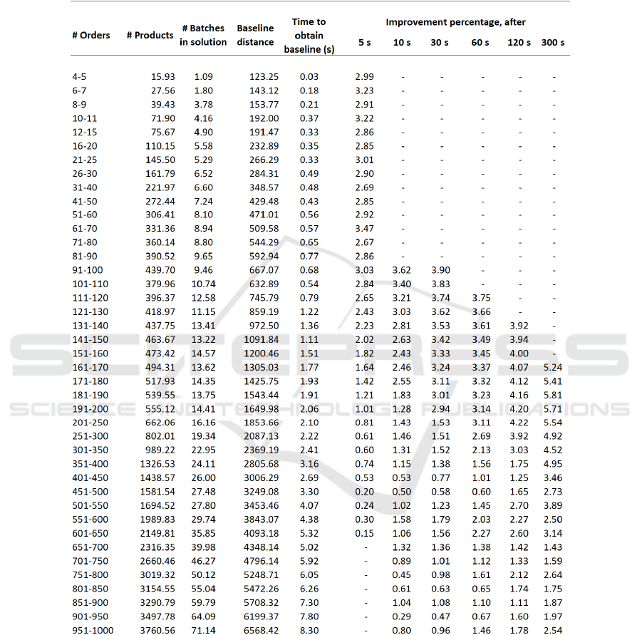
APPENDIX
Table 1: Aggregation of test-instance results into categories based on number of orders in the OBP’s. Within each category
the average over all results is shown. Whenever the optimizer (SBI) failed to obtain a result within the specified time, or when
it self-terminated, a minus sign (-) is shown. The distances shown are standardized.
Analysis of Computational Efficiency in Iterative Order Batching Optimization
353
