
Post-hoc Diversity-aware Curation of Rankings
Vassilis Markos
1
and Loizos Michael
1,2
1
Open University of Cyprus, Nicosia, Cyprus
2
CYENS Center of Excellence, Nicosia, Cyprus
Keywords:
Diversity, Preferences, Ranking, Shuffling.
Abstract:
We consider the problem of constructing rankings that exhibit a prescribed level of diversity. We take a black-
box view of the ranking procedure itself, and choose, instead, to post-hoc curate any given ranking, deviating
from the original ranking only to the extent allowed by any given constraints. The curation algorithm that we
present is oblivious to how diversity is measured, and returns shuffled versions of the original rankings that are
optimal in terms of their exhibited level of diversity. Our empirical evaluation on synthetic data demonstrates
the effectiveness and efficiency of our methodology, across a number of diversity metrics from the literature.
1 INTRODUCTION
The over-abundance of options in practically any facet
of modern life makes it unrealistic for any individ-
ual to meaningfully consider them all. An often-used
technology-mediated solution is to present these op-
tions in a ranked manner, as in the case of receiving a
ranked list of results when posing a web search query.
Although these rankings might capture some form
of preference that is centrally defined by the technol-
ogy provider (e.g., ranking higher a well-connected
web page), it is generally the case that the preferences
expressed in rankings are adapted, through machine
learning, to the individual who is consuming the rank-
ings. Since the learning itself happens by observing
the choices that the individual makes through those
rankings, it is not surprising that this process leads to
echo chambers, where the individual and the learning
algorithm reinforce each other in a narrower and nar-
rower view of what is to be ranked (or ranked higher).
Although such echo chambers are already inher-
ently problematic, they can be even more so when
what is being ranked are other individuals. Such could
be the case, for instance, in social networking sites,
where the linear manner in which one’s “friends”
might be presented might lead, through the reinforce-
ment effect mentioned above, to one interacting with
only a “selected few”, exacerbating social stereotyp-
ing, biases against minorities, and discrimination.
Such considerations are particularly relevant in the
context of the EU-funded project “WeNet: The In-
ternet of Us”, which seeks to design and develop a
machine-mediated platform that connects a requester
with potential volunteers who can help the former ad-
dress a given task. To reduce the risk of the aforemen-
tioned issues arising, the project embraces diversity-
awareness as a core principle in machine-mediation.
Diversity-awareness should not be taken to imply
that maximum diversity is always desirable; instead,
it implies that diversity should be carefully balanced
in each particular context. Indeed, deciding when di-
versity should be promoted to ensure inclusion, and
when it should be restricted to ensure protection, is
an ethically-challenging question (Helm et al., 2021).
Accordingly, this work takes the position that how
diversity is measured, and the level of diversity that
should be exhibited by a ranking, are externally deter-
mined and given. Our proposed approach seeks, then,
to demonstrate how that diversity can be achieved by
curating a given ranking. The ranking itself is also as-
sumed to be externally determined, which in the case
of the WeNet project would correspond to a ranking
expressing the user’s preferences, as learned by ob-
serving the user interact within the WeNet platform.
Since deviating considerably from this given ranking
(while promoting or restricting the level of diversity
with respect to what is already present) would antag-
onize the purpose of having a user-specific ranking to
begin with, we assume that we are provided with con-
straints on what constitutes an acceptable deviation.
Given the above, our proposed curation algorithm
proceeds to shuffle the given ranking, while respect-
ing the given constraints, towards achieving a level of
diversity that is as close to the given specifications as
Markos, V. and Michael, L.
Post-hoc Diversity-aware Curation of Rankings.
DOI: 10.5220/0010839600003116
In Proceedings of the 14th International Conference on Agents and Artificial Intelligence (ICAART 2022) - Volume 2, pages 323-334
ISBN: 978-989-758-547-0; ISSN: 2184-433X
Copyright
c
2022 by SCITEPRESS – Science and Technology Publications, Lda. All rights reserved
323

possible. We prove that the algorithm returns optimal
rankings, in a formally specified sense, and we empir-
ically demonstrate its effectiveness and efficiency.
2 RELATED WORK
In what follows we review some of the most widely
used ranking methodologies and metrics of diversity.
2.1 Ranking Methodologies
An early but popular learning-to-rank methodology is
RankNet (Burges et al., 2005), where a Neural Net-
work learns a ranking function from observed pairs
(A,B) that are labeled by target probabilities P
AB
that
A is preferred over B. RankNet uses a probabilistic
ranking cost function based on the target probabilities,
which it seeks to minimize using gradient descent.
A well-known variant of RankNet is DirectRank
(K
¨
oppel et al., 2019), which seeks to learn a quasi-
order (i.e., reflexive, anti-symmetric, transitive) re-
lation over an attribute space by observing pairwise
comparisons of attributes. Since this is beyond what
a standard Neural Network could do, DirectRank em-
ploys two identical Neural Networks that are trainable
on pairwise comparisons, and appropriately enhances
them and combines their outputs via an extra neuron.
In (Cakir et al., 2019), another Neural Network
based learning-to-rank methodology, FastAP, is pre-
sented. FastAP is a Deep Learning method that is
based on an algorithm that computes Average Preci-
sion (AP) significantly faster than other approaches
— average precision is defined as the (continuous or
discrete, accordingly) convolution of ranking preci-
sion with ranking recall. The architecture of FastAP
relies on learning a Deep Neural Network that maps
entities into a d-dimensional Euclidean space and is
optimized for AP. The contribution of the above work
is mostly focused on two axes: (i) a new significantly
faster way to compute AP given a ranking is provided,
based on discretizing the underlying convolution and
using a histogram-based approach and; (ii) introduc-
ing a new learning strategy regarding mini-batching,
were batches are collected so as to form difficult prob-
lems — i.e., they contain, among others, some highly
similar entities — so as to reduce time complexity
(namely, introducing harder learning examples helps
avoiding larger batches during the training phase).
In (Pfannschmidt et al., 2018), there are presented
two neural-based context-sensitive ranking method-
ologies that allow for a ranking to take into account
information regarding the ranked items and possible
underlying relations. The two methodologies pre-
sented, First-Aggregate-Then-Evaluate-Net (FATE-
Net) and First-Evaluate-Then-Aggregate-Net (FETA-
Net), both rely on computing a ranking score function
which maps pairs of the form (a,A), where a is an en-
tity and A a set of entities (i.e., a context), to a rank-
ing score. The difference between FETA and FATE is
that in FETA all scores for each entity are computed
using a ranking function that takes into account pair-
wise (in the simplest case) dependencies between en-
tities, while in FATE, a representative for each context
is computed first, followed by the computation of the
ranking scores, according again to a context depen-
dent ranking (utility) function. (Oliveira et al., 2018)
present a ranking/comparison methodology which re-
lies on the analysis of paired comparison data. The
novelty introduced by (Oliveira et al., 2018) is that,
in contrast to other works, the comparison function
— i.e., the function used to infer whether a is more
preferred than b — is assumed to be only partially
known. Namely, it is assumed that the comparison
function belongs in a class of functions and make no
other assumptions regarding its form — in the ex-
periments presented in (Oliveira et al., 2018), this
class consists of all the functions whose inverse is a
polynomial of some certain degree with a bounded
support. Given the above assumptions, a new com-
parison/ranking methodology is presented, PolyRank,
which transforms the comparison learning problem
into an efficiently solvable Least-Squares problem.
Perhaps the most close in spirit to our work is
the learning-to-rank approach PRM (Personalized Re-
ranking Model) (Pei et al., 2019). PRM is a method-
ology that relies on re-ranking ranked lists accord-
ing to personalized criteria for a certain user. Like
our work, PRM can be appended on top of any rank-
ing methodology. Unlike our work, however, which
simply receives a ranked list, PRM expects to receive
ranking scores for each entity in an attribute space. It
takes into account the output of the ranking process
as well as relations among the ranked entities and the
user’s preferences/history (explicitly described) and
re-computes ranking scores, thus yielding a new rank-
ing that adheres to the user’s personal preferences.
2.2 Diversity Metrics
In this subsection we shall present in detail ways
in which diversity may be quantified. To begin
with, measures of diversity have been widely stud-
ied, especially within the context of Ecosystem Biol-
ogy as well as in other fields, such as business hu-
man resources management. Hence, there are nu-
merous metrics that measure diversity from certain
ICAART 2022 - 14th International Conference on Agents and Artificial Intelligence
324

viewpoints and under certain assumptions. Here we
will discuss many already existing metrics as well as
present ways in which they could be utilized during a
ranking process with diversity in mind.
Starting with basic metrics, the most common one
is richness (Colwell, 2009), defined as the number of
different classes present in a certain sample of entities
S. More formally, richness(S), is defined as follows:
richness(S) := #{p ∈ P : p ∩ S 6= ∅}. (1)
A normalized version of richness, where we divide by
the total number of classes in X, is the following one:
richness(S) :=
richness(S)
#P
. (2)
As one may observe, richness captures only
vaguely one of the many meanings diversity has in
everyday language as well as in several applications.
A simple way to obtain more meaningful informa-
tion regarding a sample’s diversity is through the
so-called Berger-Parker Index, BP(S), (Berger and
Parker, 1970), which corresponds to the maximum
abundance ratio of S, i.e.:
BP(S) := max
i=1,...,n
p
i
, (3)
where S is assumed to be partitioned into classes
{C
1
,...,C
n
} and p
i
:=
#C
i
/#S, i = 1,...,n, are the cor-
responding relative frequencies. In order to facilitate
comparison with other metrics we will discuss later
on, we shall use the following version of BP(S) which
is increasing with respect to sample diversity:
BP(S) := 1 − BP(S). (4)
Another way to measure diversity is to introduce
more sophisticated metrics, such as Simpson’s Index
(Simpson, 1949) — often referred to as Herfindahl-
Hirschmann Index (HHI) in economics (Herfindahl,
1950). Simpson’s index, given a sample, S, parti-
tioned into classes {C
1
,...,C
n
}, represents the prob-
ability two randomly chosen entities to belong to the
same class. So, if p
i
, i = 1,. . . , n, are the relative fre-
quencies of all classes, C
i
, as above, then Simpson’s
Index, λ(S), equals:
λ(S) :=
n
∑
i=1
p
2
i
. (5)
In the same probabilistic view of diversity, one
may also define Shannon’s Index (Spellerberg and Fe-
dor, 2003), which coincides with Shannon’s entropy,
i.e.:
H(S) := −
n
∑
i=1
p
i
ln p
i
. (6)
The idea of Shannon’s Index is that, the more uni-
formly distributed sample entities are, the more di-
verse a sample should be considered, since it is more
difficult to guess to which class a randomly drawn en-
tity would belong (Shannon, 1948). Indeed, Shan-
non’s Index is equal to 0 in cases where all classes but
one are empty, while it attains its maximum value,
lnn, for p
i
=
1
/n, i = 1,...,n.
A natural normalization would be to divide H(S)
by its maximum value, ln n, obtaining the following
normalized version of Shannon’s Index:
H(S) :=
H(S)
lnn
. (7)
Other more complex metric of diversity are the so-
called Hill numbers (Hill, 1973). Hill numbers are
given by the following formula, where q is a parame-
ter of the metric:
q
D(S) :=
n
∑
i=1
p
q
i
!
1
/1 − q
. (8)
Observe that for q = 1, equation (8) cannot be com-
puted, in which case we compute the corresponding
limit as q → 1, as shown in equation (9)
1
D(S) := e
H(S)
. (9)
The above metric, also referred to as effective number
of species, true diversity or gamma-diversity in Biol-
ogy, corresponds to the number of equally abundant
classes required to achieve the same average propor-
tional abundance as in S (Chao et al., 2010; Colwell,
2009).
While Hill numbers are used in Biology to mea-
sure species diversity at a global scale, there also other
metrics that allow for computing diversity at a more
local scale — e.g. in smaller natural habitats or in
local departments of businesses. One of the most
popular choices is alpha-diversity, (Whittaker, 1960),
which is defined as follows:
q
D
α
(S) :=
k
∑
i=1
n
∑
j=1
p
i
p
q−1
j|i
!
1
/1 − q
. (10)
In the above, n is the total number of classes, as pre-
viously, while k corresponds to the total number of
local components — e.g., local habitats. Also, p
j|i
is the relative frequency of class C
j
at component i
while p
i
is the relative size of component i in S. Based
on alpha diversity, which is of local nature, another
popular diversity metric is beta-diversity, (Whittaker,
1960; Tuomisto, 2010), which is defined as the ratio
between total and local diversity, namely:
q
D
β
(S) =
q
D(S)
q
D
α
(S)
. (11)
Another conceptualization of diversity is under-
standing diversity as the opposite of similarity. In this
Post-hoc Diversity-aware Curation of Rankings
325

sense, a natural choice could be to define diversity of
a given sample S as:
div(S) :=
∑
1≤i< j≤#S
w
i j
sim(x
i
,x
j
)
2
. (12)
In the above, sim is any (normalized) similarity met-
ric defined on S and w
i j
are non-negative weights that
sum to 1, while x
i
,x
j
∈ S. Some choices for sim,
among others, could be L
p
metrics, cosine similarity,
etc.
3 POST-HOC SHUFFLING
In this section we present and discuss an abstract
framework that shuffles a given ranking to improve
its diversity according to a given metric µ. We start
by presenting an unconstrained version of the algo-
rithm where the shuffled ranking can differ arbitrarily
from the initial ranking, and then show how to extend
that to obey given constraints.
Let X = {x
1
,...,x
n
} be a finite set and consider
a ranking function r, i.e., a function that maps X to
a vector r(X). Now, let us assume that µ is a certain
metric we would like to monitor in r(X) — e.g., the
diversity of some part(s) of the returned ranked list.
More precisely, let without loss of generality µ take
values in [0,1] and let D ∈ P ([0,1])
n
be a sequence
of sets of µ’s desired values for each initial part of a
ranking r(X ) of the elements of a set X. For instance,
D in case of a set X = {x
1
,x
2
,x
3
,x
4
} could have the
following form:
D = ({0.47}, [0.33, 0.65], {0.56, 0.89}, {1}) . (13)
So, if r(X) = (x
3
,x
2
,x
4
,x
1
) is a ranking of X, D
informs us that it is desired that µ(r(X )
1
) = 0.47,
µ(r(X )
2
) ∈ [0.33,0.65], µ(r(X )
3
) ∈ {0.56,0.89} and
µ(r(X )
4
) = 1, where by r(X)
i
we denote the list con-
taining the first i elements in r(X ).
Then, given a set X = {x
1
,...,x
n
} and a ranking,
r(X ), of it, we would like to shuffle r(X) or, equiv-
alently, provide an alternative ranking r
∗
such that
each initial part r
∗
(X)
i
of r
∗
(X) satisfies the condi-
tion µ(r
∗
(X)) ∈ D. However, it is not difficult to see
that this is not possible in most cases. So, a more
realistic goal would be to demand that r
∗
(X) is not
globally inferior to any other ranking r(X). Formally,
we first define D-loss, L
D
(r
∗
), or simply L(r
∗
) when
D is obvious from the context, as follows:
L(r
∗
) := (dist(µ(r
∗
(X)
i
),D
i
))
n
i=1
. (14)
That is, L(r
∗
) is the sequence of distances of µ com-
puted at each initial part of r
∗
(X) from D
i
(the i-th set
in D). Given that, we shall say that a ranking r
1
dom-
inates another ranking r
2
if the following two condi-
tions hold:
L(r
1
)(i) ≤ L(r
2
)(i), for every i ∈ {1, . . . , n} (15)
L(r
1
)(i
0
) < L(r
2
)(i
0
), for some i
0
∈ {1, . . .,n} (16)
Given the above definition, a reasonable goal would
be to compute a shuffled ranking r
∗
that is not dom-
inated by any other shuffled ranking r
0
in the above
sense; i.e., the shuffled ranking r
∗
is Pareto optimal.
A simple method to determine r
∗
is given by Al-
gorithm 1, where at each iteration we compute the
next element of r
∗
(X) by sorting all unranked ele-
ments of X by ascending distance from D
i
, dist(µ(X \
r
∗
(X)), D
i
), and appending the first element of that
list to r
∗
(X). Sorting is performed according to Algo-
rithm 2.
Algorithm 1: Diversity-aware shuffling.
1: procedure SHUFFLE(X, µ, D)
2: µRank ← ∅
3: for i = 1, . . . , X.length do
4: x
∗
← SORTBY(X,µRank,µ,D
i
)[0]
5: µRank[i] ← x
∗
6: end for
7: return µRank
8: end procedure
Algorithm 2: SORTBY sorting algorithm.
1: procedure SORTBY(X, µRank,µ,D
i
)
2: dists ← ∅ Empty dictionary.
3: for x ∈ X \ µRank do
4: dists[x] ← dist(µ(µRank ∪ {x}),D
i
)
5: end for
6: return dists.sortByValue() Sort keys.
7: end procedure
Algorithm 1 performs a greedy search for the best
candidate to append next to the generated ranking as
described above. At this point we should remark that,
while SHUFFLE does not take the ranking function r
into account, is utilized in SORTBY at each iteration
as a tie-breaker. That is, from all the possible x ∈ X
that may satisfy x = argmin
x∈X\µRank
dist(µ(µRank ∪
{x}),D), we prefer the one ranked higher by r.
In the following lemma we state two obvious, yet
important, properties that the returned ranking, µRank
has:
Lemma 1. Given a set X = {x
1
,...,x
n
}, a ranking
function r, a metric µ and a sequence of desired val-
ues of µ, D, SHUFFLE as described in Algorithm 1
returns a ranking r
∗
(X) which satisfies the following
ICAART 2022 - 14th International Conference on Agents and Artificial Intelligence
326

two conditions:
dist(µ(r
∗
(X)
1
),D) = min
x∈X
dist(µ({x}),D
1
) (17)
dist(µ(r
∗
(X)
i
),D) = min
Y ⊆X , #Y=i
r
∗
(X)
i−1
⊆Y
dist(µ(Y ),D
i
) (18)
for each i = 2,...,n.
Proof. Regarding r
∗
(X)
1
, it is chosen in order to sat-
isfy (17). Now, for some i ≥ 2 we observe that if
Y ⊆ X is such that #Y = i and r
∗
(X)
i−1
⊆ Y , then,
again, r
∗
(X)
i−1
∪ {x
∗
} — where x
∗
is determined as
in Algorithm 1 — satisfies the following inequality:
dist(µ(r
∗
(X)
i−1
∪ {x
∗
}),D
i
) ≤ dist(µ(Y ),D
i
). (19)
So, r
∗
satisfies both (17) as well as (18).
Using the above, we may now prove the follow-
ing:
Theorem 1. Given a set X = {x
1
,...,x
n
}, a ranking
function r, a metric µ and a sequence of desired val-
ues of µ, D, SHUFFLE returns a ranking r
∗
(X) that is
Pareto optimal.
Proof. Follows directly from Lemma 1.
As one may easily observe, the above method fa-
vors µ over r. That is, we only utilize our initial rank-
ing as a tie-breaker — which could naturally lead to
completely ignoring r in case no ties occur — while
we focus on keeping µ as close as possible to the set of
desired values, D. While in some scenarios this may
be our target behavior, there are also cases where pre-
serving µ is only a secondary objective compared to
yielding an accurate ranking according to some given
ranking function, r. A natural solution to this issue
is to allow for a strict constrain capturing how r
∗
(X)
can deviate from r(X), let us denote it by R(r
∗
,r) or
simply R.
Before we proceed with the rest of our framework,
we shall remark at this point that we consider restric-
tions R that are monotonic with respect to the involved
rankings’ initial parts in the following sense: if R is
violated for some initial part r
0
(X)
i
of r
0
(X), then it
is also violated for each initial part r
0
(X)
j
for j > i.
This demand, while restricting the possible choices
for R, is aligned with the idea that when it comes to
ranking, it is the first positions that matter the most,
so we would like to exclude the case where a ranking
violates R in some initial positions while it does not
entirely do so.
So, instead of returning a ranking, r
∗
, that is
Pareto optimal among all the possible rankings, we
seek to compute a ranking, r
∗
, that is Pareto optimal
among all possible rankings that respect R.
In this direction, we can design a variation of Al-
gorithm 1 that yields a shuffled ranking that respects
R and at the same time is Pareto optimal, in the above
setting. Namely, given a set X, a ranking function r,
a metric µ, a sequence of sets of desired values of µ,
D, as well as a deviation restriction R, we aim to find
a ranking r
∗
(X) such that µ(r
∗
(X)) is close to D —
where “close” is understood in the context of Pareto
optimality — and at the same time r,r
∗
do not violate
R. This is achieved by Algorithm 3, which is actu-
ally a backtracking search for r
∗
, with R serving as
the backtracking condition.
Algorithm 3: Constrained diversity-aware shuffling.
1: procedure SHUFFLE2(X,r,µ,D,R)
2: rank ← r(X)
3: µRank ← ∅
4: i ← 0
5: f ront ← SORTBY(X, µRank,µ,D
i
) Stack.
6: while f ront 6= ∅ do
7: next ← f ront.pop()
8: µRank.append(next)
9: i ← i + 1
10: if R(µRank, rank) is violated then
11: µRank.pop()
12: i ← i − 1 Backtrack.
13: else if X \µRank = ∅ then
14: return µRank Found shuffling.
15: else
16: children ← SORTBY(X, µRank,µ,D
i
)
17: f ront.push(children.reverse())
18: end if
19: end while
20: return False Failed to find shuffling.
21: end procedure
We shall now make some remarks regarding Algo-
rithm 3. To begin with, observe that, when expanding
our partial ranking, µRank, we push all elements re-
turned by SORTBY in reverse order so as to ensure
that the most fitting item computed by SORTBY is ex-
amined first. Also, SHUFFLE2 is actually an extension
of SHUFFLE since, in case we set R to be a restriction
that may never be violated, then Algorithm 3 returns
the same shuffling of X that Algorithm 1 would re-
turn.
As one may expect, we can prove that, indeed,
µRank lies on the Pareto Frontier. Namely, we have
the following:
Theorem 2. Given a set X = {x
1
,...,x
n
}, a ranking
function r, a metric µ and a sequence of desired values
of µ, D, SHUFFLE2 returns a ranking r
∗
(X) such that
r
∗
is Pareto optimal among all rankings r
0
∈ R (X)
that respect R(r
0
,r).
Post-hoc Diversity-aware Curation of Rankings
327

Proof. We will proceed with reductio ad absurdum.
Let a ranking r
0
such that all the above three condi-
tions hold and, specifically, let i
0
be the minimum in-
dex such that:
dist(µ(r
0
(X)
i
0
),D
i
0
) < dist(µ(r
∗
(X)
i
0
),D
i
0
). (20)
Since we also have that:
dist(µ(r
0
(X)
i
),D
i
) ≤ dist(µ(r
∗
(X)
i
),D
i
) (21)
for every i = 1,...,n and i
0
is the minimum index
such that the inequality in (21) is strict, we have that
for every i = 1,...,i
0
− 1 it holds:
dist(µ(r
0
(X)
i
),D
i
) = dist(µ(r
∗
(X)
i
),D
i
) (22)
Equation (22) means that calling SORTBY with
X, r
∗
(X)
i
0
−1
,µ and D
i
0
as arguments yields a list
where all elements of r
∗
(X)
i
0
−1
∪r
0
(X)
i
0
−1
are ranked
below the i
0
-th element in r
0
(X), let x
0
. Furthermore,
Equation (20) ensures that x
∗
is ranked higher in the
returned list than x
∗
6= x
0
, where by x
∗
we denote the
i
0
-th element of r
∗
(X). However, this means that
(see Algorithm 3, line 7) x
0
is processed prior to x
∗
,
so, since x
0
is not the i
0
-th element of the returned
ranking, r
∗
(X), we infer that R is violated by r
0
(X)
i
0
.
which is a contradiction, since R(r
0
,r) is assumed to
hold. So, r
∗
satisfies indeed all three conditions.
So, SHUFLE2 computes, indeed, a shuffling of
r(X ) that, given R, is optimal with respect to all other
soft restrictions about µ.
4 EXPERIMENTS
In this section we shall present some experiments con-
ducted on synthetic data with our main purpose being
studying Algorithm 3 and its behavior with respect
to its hyperparameters on the special case where µ is
some diversity metric. Namely, we examine the scala-
bility of Algorithm 3 as well as how different choices
of D and R affect its behavior — either combined or
separately. At first we present our data generation
protocol and then we proceed with explaining which
specifications we decided to make to our framework.
At last, we present and discuss the results of our ex-
periments.
4.1 Data Construction
In these experiments, we study our diversity aware
ranking framework with two goals in mind: (i) to ex-
amine the effect the choice of our framework’s hy-
perparameters has on its behavior and; (ii) to exam-
ine any differences the diversity metrics we have pre-
sented may have in practice. For the purposes of
these experiments, we have generated two synthetic
datasets, P
1
and P
2
. Regarding P
1
, it consists of N
randomly generated samples of points in [0,1]
2
. and
each sample is generated under the following proto-
col:
1. At first, a set of M points in [0,1]
2
, call it C, is
generated — the points in C will serve as cluster
centers.
2. Then, for each cluster center, c
k
, in C, a sam-
ple of n
k
points is generated, under a uniform
distribution on the
1
sphere with center c
k
and radius r
k
:=
1
2
min
i6=k
∞
(c
k
,c
i
). Also, we
choose n
k
randomly from a triangular distribution
Trig(n
min
,n
max
) with mode δ =
n
min
+n
max
2
.
We chose for n
k
to be a random variable since having
clusters of fixed size would have direct implications
for our dataset’s diversity according to most met-
rics. Specifically, in our experiments, we set M = 4,
n
min
= 0 and n
max
= 10. That is, P
1
contains 10 clus-
ters with each cluster containing from 0 to 40 points.
Now, given the above data, we assign to each sample
S of D a randomly chosen target point t(S) ∈ [0,1]
2
,
which will serve as the target point of each ranking,
as we shall present below.
Regarding P
2
, it is significantly larger than P
1
,
since it consists of 17 sets, with each set containing
N = 10 samples, as in P
1
. However, while in P
1
we did
not monitor the total number of points in each sample
— i.e., each sample in P
1
may contain from 0 to 400
points — we did so in all samples in P
2
. Namely, ev-
ery set of samples in P
2
contains samples with exactly
K elements, where K = 15, 20, . . . , 95. Then, given
K we determine how many elements each of the five
clusters of a sample contains by randomly selecting a
partition of K into five non-negative integers.
4.2 Empirical Setting
Our shuffling framework, as described above is quite
abstract, so, we needed to make some specifications
in order to implement and test it. To begin with, we
chose our deviation restriction, R, to be a simple ex-
pression of the form d(r
∗
,r) ≤ d
max
, where d is a
metric defined on permutations (rankings) and d
max
is some fixed threshold provided to our algorithm.
Namely, we chose the
1
metric, which is defined as
follows:
1
(r
1
,r
2
) :=
n
∑
k=1
|r
1
(k) − r
2
(k)|. (23)
So, for instance, for n = 5, let two rankings of
X = {1, 2, 3, 4,5} be r
1
= (3, 5, 1, 4, 2) and r
2
=
(3,5,2,4,1). Then, have
1
(r
1
,r
2
) = 2 while, if r
3
=
ICAART 2022 - 14th International Conference on Agents and Artificial Intelligence
328

(4,1,3,2,5), we have
1
(r
1
,r
3
) = 12. We preferred
1
over other permutation metrics, mostly due to its
simplicity and intuitive interpretation in the context
of ranking — i.e., the total “displacement” of each
entity.
At this point we should mention that across all ex-
periments we chose to use a normalized version of the
1
metric. Namely, for given n,
1
in S
n
attains a max-
imum value of
l
n
2
−1
2
m
, so the normalized
1
distance,
denoted by
ˆ
1
, is defined follows:
ˆ
1
(r
1
,r
2
) :=
1
l
n
2
−1
2
m
1
(r
1
,r
2
). (24)
Regarding the metric µ used, we used the diversity
metrics shown in Table 1. We did not include α and
β diversities in our study since our datasets did not
have a structure that would allow us to do so. We also
chose to exclude Hill numbers since in the most used
cases in bibliography, q is set to either 0, or 1 or 2,
(Chao et al., 2010), which in each case reduces to a
function
1
of some of the metrics presented in Table 1.
Table 1: Diversity metrics used in A Series Experiments.
Method Tag
Richness R
Berger-Parker Index BP
Simpson’s Index λ
Shannon’s Index H
Another parameter that needed to be specified was
D, for which we considered two different scenarios:
(i) each set of D to be a singleton containing the same
value and; (ii) each set of D to be a singleton contain-
ing a randomly chosen value, with all choices being
pairwise independent.
Lastly, we chose a simple ranking function r
across all experiments, which ranked all points in a
sample by ascending distance to each sample’s target
point. As our distance in this case we preferred the
usual Euclidean Distance.
Given the above specifications, we performed the
following sets of experiments:
1. Set A consisted of experiments using dataset P
1
where we allowed for a single value for D for each
sample win [0,1] with a 0.05 step while we al-
lowed for d
max
to similarly vary from 0 to 1.
2. Set B consisted of experiments using dataset P
1
1
Namely, for q = 0,
0
D coincides with richness, for q =
1,
1
D is just a function of Shannon’s Index, namely
1
D =
exp(−H) while for q = 2,
2
D is the inverse of Simpson’s
Index (Chao et al., 2010).
where D took random sequences as values and
d
max
took values from 0 to 1 with a 0.05 step.
3. Set C consisted of experiments using dataset P
2
where D took random sequences as values and
d
max
took values from 0 to 1 with a 0.05 step.
Experiments of Set A where used to study the be-
havior of Algorithm 3 in a general setting and ver-
ify that its behavior is the expected one, as described
by Theorem 2. Regarding experiments in Set B, we
wanted again to test the behavior of Algorithm 3 but,
this time, under a more general protocol of determin-
ing D, so as to further support the results found in Set
A. Regarding Set C, we wanted to study properties of
Algorithm 3 related to scalability as well as determine
whether trends observed in smaller datasets — sets A
and B — were also present at a larger scale.
4.3 Results
We shall now present the results of our experiments.
To begin with, in Figure 1a we observe that the choice
of the diversity metric does not seem to affect the
overall computation time since average computation
times seem to be identical while minimum and max-
imum values also do not seem to differ significantly.
This was more or less expected since computing the
diversity of a set is not time-demanding when com-
pared to SHUFFLE2’s backtrack search while also all
four diversity metrics have similar time complexities.
As a result we choose to aggregate over all diver-
sity quantification methods in the rest three plots pre-
sented in Figure 1.
In Figure 1b we observe that the average execu-
tion time is quite well fitted by a straight line in log-
log axes (R
2
> 0.99), which implies that execution
time grows polynomially with respect to input size, n.
Namely, as shown in Figure 1c, the average execution
time of SHUFFLE2 in Set C was asymptotically cubic
with respect to n. Since, the worst-case complexity of
our backtrack searching algorithm is Θ(n!), having an
implementation that has a significantly lower average
time complexity is quite surprising and would require
further investigation.
One fact that could contribute to this unexpected
efficiency is that in all experiments we allowed for
d
max
to vary significantly, so, one may argue that the
low observed average time complexity is due to e.g.,
lower execution time of searches for higher values of
d
max
. However, as shown in Figure 1d, this is not
true since, while there is some expected variation of
the execution time of SHUFFLE2 with respect to d
max
,
it is not significant enough to account for a notable
decrease of average execution time.
Post-hoc Diversity-aware Curation of Rankings
329
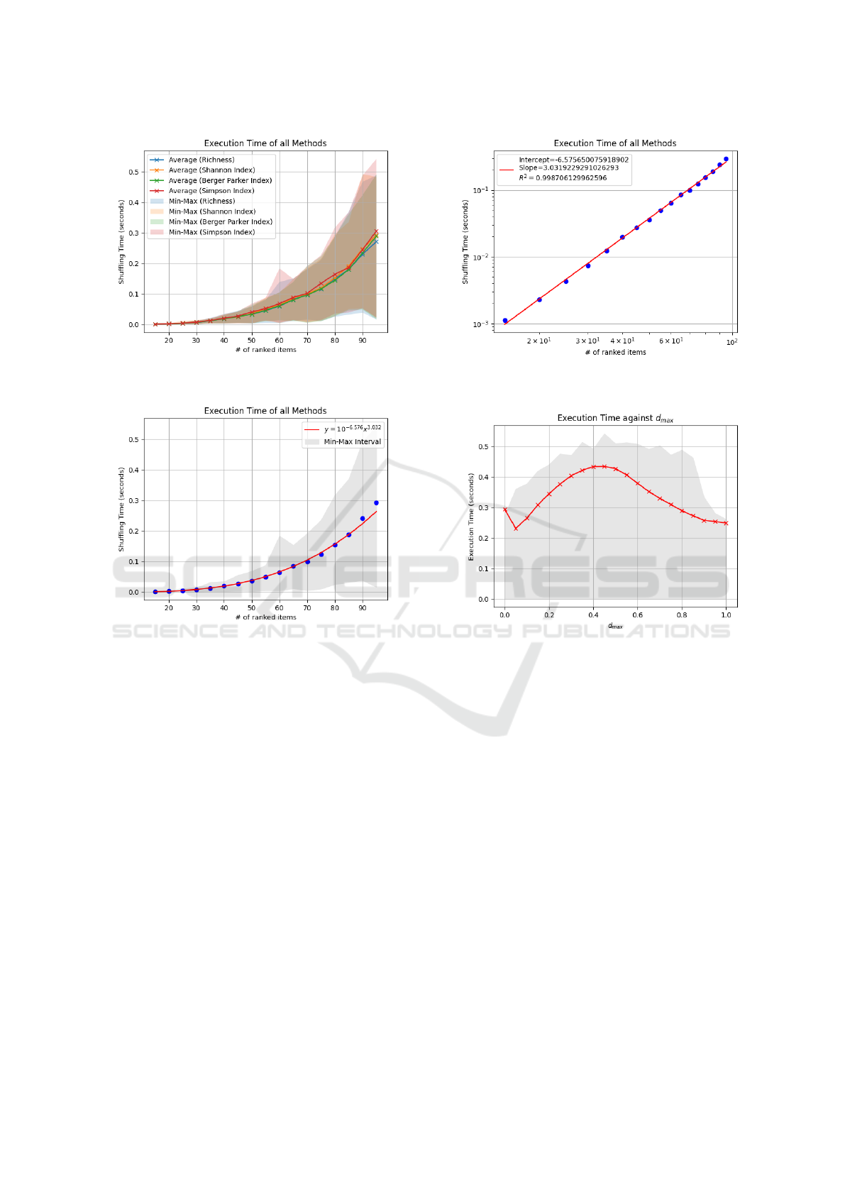
(a) Scalability of Shuffle2 with respect to all diversity
metrics.
(b) Average execution time across all diversity metrics
(Log-Log).
(c) Average execution time across all diversity metrics
alongside the fitting polynomial, y = 10
−6.576
x
3.032
.
(d) Average execution time vs deviation threshold, d
max
.
Figure 1: Scalability results regarding SHUFFLE2.
Another interesting feature observed in Figure 1d
is an initial spike for d
max
= 0. We can provide two
reasons for this spike — possibly among others. At
first, d
max
= 0 means that we have to look for the ini-
tial ranking r throughout the entire search space, so
even in this case we have to explore some possibly
significant part of the search tree. On the other hand,
in each experiment conducted d
max
= 0 was the first
case examined after the dataset was loaded, so this
initial spike might be a result of caching the dataset in
memory for the rest values of d
max
, as well.
Next, we examine how much the ranking returned
by SHUFFLE2 deviates from the initial ranking, r —
see Figure 2. Starting from Set A, we observe that
using all four metrics, the algorithm initially returns
a shuffled ranking r
∗
that seems to take as much dis-
tance allowed from r as possible, while after around
d
max
= 0.4 in all four cases of Set A the distance be-
tween r and r
∗
converges to a value around 0.6 —
Figure 2a demonstrates the case of Shannon Entropy,
while using any of the rest metrics yielded similar re-
sults. Since SHUFFLE2 for d
max
= 1 is actually Al-
gorithm 1, we also infer from the above results that
an empirical estimation of the maximum average de-
viation from the initial ranking r using Algorithm 1
is slightly above 60% as quantified using
1
as our
metric. Similarly, in the case of Set B — Figure
2b again demonstrates the case of Shannon Entropy,
while using any of the rest metrics yielded similar re-
sults — we observe the very same behavior, but for
the maximum and minimum values of
1
(r
∗
,r) which
are less diverse than those in Set A. This may be ex-
plained by the different way we have chosen D in each
case, since in Set A the values of D were ordered and
strictly determined — D was constant across all initial
parts, r
∗
(X)
i
— while in Set B it was allowed to vary
randomly with i.
At this point, observe that in both plots in Fig-
ure 2 the distance between r
∗
and r is virtually in-
creasing even past the 0.4 limit we described above.
ICAART 2022 - 14th International Conference on Agents and Artificial Intelligence
330

(a)
1
distance between r
∗
and r using Shannon’s Index
as diversity index (Set A).
(b)
1
distance between r
∗
and r using Shannon’s Index
as diversity index (Set B).
Figure 2: Results from experiment sets A and B regarding
the deviation of the returned ranking, r
∗
, from the initial
ranking, r, as measured using the
1
ranking metric.
One may have expected that a virtually unconstrained
search for the Pareto optimal shuffling would termi-
nate in more or less the same time, however, as d
max
increases, so does the part of the search graph that
SHUFFLE2 is allowed to search, which can explain
why execution time is increasing with d
max
, even if at
a slower rate after some certain point.
Since in all experiments we defined µ to be a diver-
sity metric, we will refer to D-loss as defined in Equa-
tion (14) as diversity loss. In Figure 3 we present, at
first, the average diversity loss in the first set of ex-
periments (Set A) — Figure 3a — where we observe
a similar trend across all diversity metrics — the cor-
responding curves for the rest metrics were similar to
the one shown in Figure 3a. Namely, initially L is
quite high, then it approaches zero for some of the first
initial parts of the returned ranking and, eventually, it
grows again away from zero. This behavior is repli-
cated at a larger scale in Set C — Figure 3b — where
we allowed for rankings to contain each 95 elements
— instead of 15 we present in Figure 3a. Again, av-
erage diversity loss drops for the first initial parts for
each metric while then it rises to some higher value.
The more vivid variation of average diversity loss we
observe in the results of Set C is attributed mostly to
D taking random values compared to Set A where D
took a single value across each sample. We also pro-
duced plots for the rest subsets of Set C — namely,
for rankings of length l = 15,20, . . . , 95 — but they
all were more or less truncated versions of Figure 3b.
4.4 Diversity Loss
This trend observed in Figure 3 is of special interest so
we shall further elaborate on it. As we have discussed
in the description of our framework — see Section
3 for more details — adhering to the restrictions im-
posed by D is treated as a soft restriction throughout
Algorithm 3. That is, we do not expect that the shuf-
fled ranking returned by SHUFFLE2 will be globally
optimal with respect to diversity loss, L, but, as we
proved in Theorem 2, each shuffled ranking returned
is Pareto optimal. However, as we observe in Figure
3, in all cases of diversity metrics we have a similar
trend. Namely, L is initially relatively high, it then
drops close to zero for the first initial parts of the re-
turned ranking and then it rises again away from the
desired levels of diversity determined by D for the last
parts of the returned shuffled ranking.
The above behavior is expected, given the metrics
we have at our disposal. To begin with, given a set,
X, and a a diversity metric, µ, each ranking of X, let
r(X ), has the same diversity as X since none of the
metrics we used is sensitive to the order in which el-
ements appear in X — this is a natural feature of a di-
versity metric since it quantifies the diversity of a pop-
ulation/sample at a given time/time interval. Also, as
we include more of X’s elements into our ranking we
expect µ(r(X)
i
) to be approximately div(X) since, for
large sets, introducing another element does not affect
diversity dramatically — at least not when quantify-
ing it using the metrics discussed in Section 2.2. As a
result, we are not able to guarantee adherence to D
i
as
far as large values of i are concerned, which is clearly
depicted in all figures in Figure 3. Also, the same ap-
plies to singletons, since the diversity of a singleton
takes some trivially constant value under all the met-
rics presented in Section 2.2.
Post-hoc Diversity-aware Curation of Rankings
331

(a) Average diversity loss (L) using Shannon’s Index as
diversity metric (Set A).
(b) Average diversity loss (L) using Shannon’s Index as
diversity metric (Set C).
Figure 3: Average Diversity Loss (L) across experiments of sets A and C.
So, the only values of i for which we could rea-
sonably expect that µ(r
∗
(X)
i
) ≈ D
i
are those closer to
bur larger than 1. As shown in Figure 3, this is in-
deed the case since, using any metric, we achieve a
minimum diversity loss for such values of i. At this
point we should also observe that the fact that each
ranked sampled contains elements from (at most) four
classes plays an important role. Namely, with less
than four — or richness(X), in general — items the
values diversity may take — with any metric but for
richness in mind — are more restricted than when
there are more — but not much more — items in the
sample. Intuitively, this happens because, especially
when richness(X) is not large, modifying the diver-
sity of a sample boils down to adding a few items
to it. On the contrary, when there are too few items
in a sample, diversity values are more “sparsely” dis-
tributed in [0, 1] while when the cardinality of a sam-
ple is much larger than richness(X), adding a few
items does not significantly affect its diversity. Bear-
ing these in mind, it is expected that a sample is more
flexible in manipulations of its diversity when it con-
tains roughly as many items as the classes available.
Less items lead to less flexibility as well as much
more.
This trend is also reflected in the distance the rank-
ing r
∗
returned by Algorithm 3 has from r, as shown
in Figure 2. Namely, for tighter values of d
max
we
observe that r
∗
takes as much distance as possible
in order to minimize diversity loss as much as pos-
sible. In these cases there is an expected trade-off be-
tween adherence to r and diversity, which is attributed
mostly to the following two factors: (i) first, the rank-
ing methodology we chose in all our experiments was
promoting similarity in the first positions of the re-
turned rankings while, at the same time it compro-
mised diversity and; (ii) second, diversity is inher-
ently opposite to similarity in the sense that a set that
is considered diverse should contain elements that are
dissimilar to each other above some certain threshold.
Bearing in mind the above, we can easily explain the
observed trade-off between diversity and adherence to
the initial ranking we provide to SHUFFLE2.
To shed more light on the above behavior
of SHUFFLE2 let us consider a setting where
X = {a
1
,a
2
,a
3
,b
1
,b
2
,b
3
}, where a, b denote the
classes of the corresponding elements and r(X ) =
(a
1
,a
2
,a
3
,b
1
,b
2
,b
3
). Also, let us consider that we
measure diversity using Richness and that our de-
sired diversity values are D = (1,1,1,0, 0, 0), i.e., we
care about the first half of the list being highly di-
verse while we have no demands regarding the list’s
last elements. Then, it is not difficult to see that
any ranking, r
∗
(X), containing at least one a and
at least one b would yield a diversity loss vector
L(r
∗
) = (1,0,0, 0, 0, 0). However, a ranking such as
r
∗
(X) = (a
1
,b
1
,a
2
,a
3
,b
2
,b
3
) has an
1
distance from
r(X ) equal to
1
(r
∗
,r) =
1+2+3
17
≈ 0.353. That is, in
order to achieve a highly diverse shuffling, we had to
deviate from our initial ranking at about 35%.
5 DISCUSSION
Our work raises certain issues and suggests possible
directions for future work that we discuss below.
5.1 Determining D in Practice
Our developed framework assumes that D, the desired
level of diversity, is externally provided, with each of
ICAART 2022 - 14th International Conference on Agents and Artificial Intelligence
332

its components, associated to an initial part of the con-
structed ranking, being a set or interval of values. Al-
though we have not fully explored this flexibility in
our empirical setting, both of these features could be
useful in practical applications, where one would at-
tempt to actually determine what D should be.
A first approach to determining D could be to
measure the diversity µ(X) of the set X of options
that are available, and set each component of D to
equal {µ(X )}. This would effectively ask for some
form of uniformity of the diversity exhibited in any
initial part of a ranking presented to the user. Thus,
the user would not only wish for the entire list of op-
tions presented to them to be diverse, but also for the
first handful of results in that ranking — which prac-
tically is what a user gets to see when making their
choice — to also be equally diverse.
Variations are, of course, possible. Instead of in-
sisting on uniformity, the user could ask that each ini-
tial part of the ranking is at least as diverse as the en-
tire list by setting each component of D to equal the
interval [µ(X),1], so that the shuffling algorithm will
not seek to demote diversity of a part of the ranking
if this happens to be higher than µ(X). Analogously,
the user may wish to relax the minimum bound on the
diversity and replace the interval [µ(X), 1] with, say,
[µ(X)/2, 1], insisting that some diversity is minimally
and uniformly required in each part of the ranking.
An interesting direction for future research would
be to determine D using actual user feedback in real
scenarios. Namely, it would be interesting to see to
what extent and under what conditions users desire
ranked lists presented to them to be diverse and, on
top of that, what part of the list is of significant im-
portance — for instance, in typical web search tasks,
the first page of the returned results is usually of the
highest significance to a user.
One approach to learning the diversity that a user
may be seeking in their ranked options is to track the
user’s past choices from ranked lists. The precise
choice from each specific ranking can, naturally, be
used as a signal of how the user wishes the options to
be ranked to begin with. But in addition, looking at
the choices C
t
of the user after t rounds of being pre-
sented with a ranking and making a choice, one could
consider the diversity µ(C
t
) of C
t
as an indication of
the level of diversity that the user would wish to see
in subsequent rounds of rankings. Setting each com-
ponent of D to equal µ(C
t
), and presumably updating
D over time as C
t
is computed for larger and larger
values of t would capture this intuition.
A more involved solution would be to maintain a
list of user choices as above, but partitioned based on
the position in the ranking of each choice made. So,
if during round t a user chooses option at position i
in their presented ranking, then that option would be
added to list C
t
i
. D would then be defined by setting its
i-th component to equal µ(C
t
i
). Further accounting for
the amount of data within each list C
t
i
of choices, one
could insist that each component of D is some confi-
dence interval around µ(C
t
i
), whose size is determined
by the size of C
t
i
. This would then be able to capture
situations where a user might signal that different lev-
els of diversity are desired for different initial parts
of the ranking; e.g., no diversity preference for the
first handful of results (so that the original ranking is
maintained), but then maximum diversity in the sec-
ond handful of results (so that the user can explore
alternatives that might be less preferred according to
the original ranking, but are highly diverse).
5.2 Measuring Shuffling Deviation
A choice that we made for the purposes of our em-
pirical evaluation was to implement the deviation re-
striction, R, required by Algorithm 3, through the use
of
1
as a simple to compute yet informative way to
quantify distance between two ranked lists. As we
explained in Section 4.2,
1
is naturally interpreted
as the total “displacement” required to transit from a
ranking r
1
to another ranking r
2
. However, what mat-
ters in most occasions a ranking is used, is the first
part of the returned ranked list. So,
1
may not be the
most appropriate choice since it does not make a dis-
tinction between changes in the first, middle or last
places of a ranking r. A natural adaptation of
1
ac-
commodating the above is to introduce weights, w
k
,
∑
n
k=1
w
k
= 1, such that moving the first, say, element
of r(X) three places down the list matters more than
moving the 15
th
element to position 18.
Other than distance-based deviation constraints
that apply globally on a ranked list, it would also be
meaningful to explore more complex restrictions R,
including ones that are not necessarily based on dis-
tance metrics. For instance, in some scenarios a user
may wish to explicitly state that the initial handful of
options in the original ranking should not be shuffled
and that subsequent options could be shuffled more
the later in the ranking they appear.
5.3 Efficient Search of Shufflings
In the implementation of Algorithm 3, as used in
the empirical evaluation presented in Section 4, we
adopted a greedy breadth-first strategy to search the
space of all shufflings of r(X). The only heuristic we
have implemented in order to alter the order nodes
are expanded is, as mentioned in Section 3, that when
Post-hoc Diversity-aware Curation of Rankings
333

sorting any remaining items using SORTBY we break
any ties that may occur using r, expecting that an item
ordered at a higher position in r(X) will lead to a shuf-
fled ranking r
∗
(X) with smaller
1
distance from r.
However, there is plenty of space for further im-
provement in this direction. To begin with, SHUF-
FLE2’s performance may be enhanced by introduc-
ing Forward Checking. Since after each expansion
of the generated ranking, µRank, the remaining chil-
dren nodes are fewer than in the previous iteration,
Forward Checking may lead to significant parts of the
search tree to be pruned. Moreover, one may also de-
ploy more sophisticated search techniques such as A
∗
or other heuristic or stochastic search methods in or-
der to further reduce the running time of SHUFFLE2.
6 CONCLUSIONS
Motivated by the widespread use of ranking to fa-
cilitate the choices of individuals, and the real dan-
ger of ending up creating echo chambers with poten-
tially grave implications in social settings, this work
has proposed and empirically evaluated a post-hoc ap-
proach for the diversity-aware curation of rankings.
Our next steps include the integration of our method-
ology in the context of the WeNet platform, and its
evaluation on data coming from the platform’s users.
ACKNOWLEDGMENTS
This work was supported by funding from the EU’s
Horizon 2020 Research and Innovation Programme
under grant agreements no. 739578 and no. 823783,
and from the Government of the Republic of Cyprus
through the Deputy Ministry of Research, Innovation,
and Digital Policy.
REFERENCES
Berger, W. H. and Parker, F. L. (1970). Diversity of Plank-
tonic Foraminifera in Deep-Sea Sediments. Science,
168(3937):1345–1347.
Burges, C., Shaked, T., Renshaw, E., Lazier, A., Deeds, M.,
Hamilton, N., and Hullender, G. (2005). Learning to
Rank Using Gradient Descent. In Proceedings of the
22nd International Conference on Machine Learning,
ICML ’05, page 89–96, New York, NY, USA. Associ-
ation for Computing Machinery.
Cakir, F., He, K., Xia, X., Kulis, B., and Sclaroff, S. (2019).
Deep Metric Learning to Rank. In IEEE Conference
on Computer Vision and Pattern Recognition (CVPR),
pages 1861–1870.
Chao, A., Chiu, C.-H., and Jost, L. (2010). Phylogenetic
Diversity Measures Based on Hill Numbers. Philo-
sophical transactions of the Royal Society of London.
Series B, Biological sciences, 365:3599–609.
Colwell, R. (2009). Biodiversity: Concepts, Patterns, and
Measurement, pages 257–263. Princeton Univ. Press.
Helm, P., Michael, L., and Schelenz, L. (2021). Diversity by
Design: Balancing Protection and Inclusion in Social
Networks.
Herfindahl, O. (1950). Concentration in the US Steel Indus-
try. In Unpublished doctoral dissertation.
Hill, M. O. (1973). Diversity and Evenness: A Unifying
Notation and Its Consequences. Ecology, 54(2):427–
432.
K
¨
oppel, M., Segner, A., Wagener, M., Pensel, L., Karwath,
A., and Kramer, S. (2019). Pairwise Learning to Rank
by Neural Networks Revisited: Reconstruction, The-
oretical Analysis and Practical Performance. CoRR,
abs/1909.02768.
Oliveira, I. F. D., Ailon, N., and Davidov, O. (2018). A New
and Flexible Approach to the Analysis of Paired Com-
parison Data. Journal of Machine Learning Research,
19(60):1–29.
Pei, C., Zhang, Y., Zhang, Y., Sun, F., Lin, X., Sun, H.,
Wu, J., Jiang, P., Ou, W., and Pei, D. (2019). Per-
sonalized Context-aware Re-ranking for E-commerce
Recommender Systems. CoRR, abs/1904.06813.
Pfannschmidt, K., Gupta, P., and H
¨
ullermeier, E. (2018).
Deep Architectures for Learning Context-dependent
Ranking Functions.
Shannon, C. E. (1948). A Mathematical Theory of Com-
munication. The Bell System Technical Journal,
27(3):379–423.
Simpson, E. H. (1949). Measurement of Diversity. Nature,
163(4148):688–688.
Spellerberg, I. and Fedor, P. (2003). A Tribute to Claude
Shannon (1916–2001) and a Plea for More Rigorous
use of Species Richness, Species Diversity and the
‘Shannon–Wiener’ Index. Global Ecology & Bio-
geography, 12:177–179.
Tuomisto, H. (2010). A Consistent Terminology for Quan-
tifying Species Diversity? Yes, It Does Exist. Oecolo-
gia, 164(4):853–860.
Whittaker, R. H. (1960). Vegetation of the Siskiyou Moun-
tains, Oregon and California. Ecological Mono-
graphs, 30(3):279–338.
ICAART 2022 - 14th International Conference on Agents and Artificial Intelligence
334
