
Buildings Extraction from Historical Topographic Maps via a Deep
Convolution Neural Network
Christos Xydas
1
, Anastasios L. Kesidis
1
, Kleomenis Kalogeropoulos
2
and Andreas Tsatsaris
1
1
Department of Surveying and Geoinformatics Engineering, University of West Attica, Athens, Greece
2
Department of Geography, Harokopio University, Athens, Greece
Keywords: Building Detection, Historical Maps, Deep Learning.
Abstract: The cartographic representation is static by definition. Therefore, reading a map of the past can provide
information, which corresponds to the accuracy, technology, as well as scientific knowledge of the time of
their creation. Digital technology enables the current researcher to "copy" a historical map and "transcribe" it
to today. In this way, a cartographic reduction from the past to the present is possible, with parallel
visualization of new information (historical geodata), which the researcher has at his disposal, in addition to
the background. In this work a deep learning approach is presented for the extraction of buildings within
historical topographic maps. A deep convolution neural network based on the U-Net architecture is trained
by a large number of images patches in a deep image-to-image regression mode in order to effectively isolate
the buildings from the topographic map while ignoring other surrounding or overlapping information like
texts or other irrelevant geospatial features. Several experimental scenarios on a historical census topographic
map investigate the applicability of the method under various patch sizes as well as patch sampling methods.
The so far results show that the proposed method delivers promising outcomes in terms of building detection
accuracy.
1 INTRODUCTION
Automated retrieval of information from many
different images is a very important task. Historical
maps provide valuable information about the site,
with a chronological reference to the time they were
built. Thus, they may contain information on
topography, toponyms, and in relation to urban space,
streets, blocks, buildings, etc. It is therefore important
that this information can be extracted and be available
for analysis and identification of the urban landscape
of the past.
There are plenty of such maps (topographic,
urban) in public services and which can be a useful
source of information if one can take advantage of
them. These maps can be studied by many scientists
from a wide range of disciplines. This current study
uses as object the digitized maps of the Hellenic
Statistical Authority (ELSTAT) and was used for
inventory purposes (pre-enumeration, enumeration,
and post-enumeration). Such a sample map is
presented in Figure 1 and depicts the Settlement of
Petroupoli, which is a suburb of Athens, Greece, in
the 1971 Housing and Population Census. Its initial
size is 70 × 50 cm and its scale is 1:5000.
There are many GIS software and not only, which
provide the ability to vectorize an image. This process
can be performed either (semi) manually under the
supervision of a special user, or automatically. The
product resulting from this process, however, does
not differentiate the objects displayed on a map. That
is, linear elements are not separated from polygonal,
texts (letters, numbers) or point data.
Figure 1: Sample historical topographic map.
Xydas, C., Kesidis, A., Kalogeropoulos, K. and Tsatsaris, A.
Buildings Extraction from Historical Topographic Maps via a Deep Convolution Neural Network.
DOI: 10.5220/0010839700003124
In Proceedings of the 17th International Joint Conference on Computer Vision, Imaging and Computer Graphics Theory and Applications (VISIGRAPP 2022) - Volume 5: VISAPP, pages
485-492
ISBN: 978-989-758-555-5; ISSN: 2184-4321
Copyright
c
2022 by SCITEPRESS – Science and Technology Publications, Lda. All rights reserved
485
Therefore, in order to achieve a distinct rendering
of the objects, another approach must be implemented
that aims at the specific recognition of the desired
objects. The aim of this study is to extract the
geometry of the buildings from the above-mentioned
historical topographic maps that are initially in the
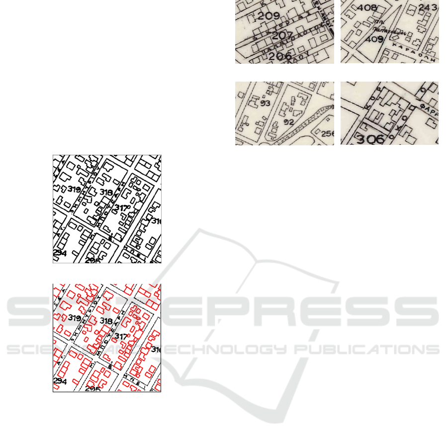
form of an image. Figure 2 shows an example of this
kind of conversion. Specifically, Figure 2(a) shows
the original binarized form of the image, while Figure
2(b) shows the footprints of the buildings, which is
the desired result. Indeed, textual information as well
as other irrelevant graphic information is effectively
isolated.
(
a
)
(
b
)
Figure 2: (a) Original binarized map subarea (b) Buildings
footprints detection.
Detecting a building footprint often becomes
difficult, as various specific challenges arise that are
usually related to the removal of background map
noise (which is common), irrelevant graphics or
textual information, etc. For example, building
geometry is often overlapped with block’s number, as
shown in Figure 3(a). In addition, there may be a
dense display of text information on the map, e.g.
street names adjacent to the lines of the building
block, free text in the map space, or either in a variety
of characters’ size, as shown in Figures 3(b) and 3(c),
respectively. In addition, there may be an overlap of
one edge of the building with the boundaries of the
building block or even two edges of the building
footprint overlapping with the block boundaries as
shown in Figure 3(d).
(a)
(b)
(
c
)
(d)
Figure 3: Building footprints detection challenges (a) Dense
textual overlapping content (b) Free text over the map (c)
Buildings footprints with varying shape, size and
orientation (d) Overlapping issues between building block
and building footprints.
In terms of buildings extraction from high resolution
aerial images, there is a variety of previous studies in
the literature (Fischer et al., 1998; Peng et al., 2005;
Dornaika and Hammoudi, 2009; Hecht et al., 2015).
However, these methodologies have limited results
on historical maps since they are considered as
significantly lower quality. In this context, (Suzuki
and Chikatsu, 2003) propose a technique for
automatic building extraction that detects rectangular
building footprints that are described by their four
corner coordinates. In another work, (Laycock et al.,
2011) represent the extracted buildings as non-
intersecting closed polygons. Recently, deep learning
approaches have attracted significant attention since
they provide state-of-the-art results (Liu et al., 2017).
Specifically, Convolutional Neural Networks
(CNNs) are deep architectures that are able to find
complicated inherent structures by transferring
features through multiple hidden layers in a non-
linear fashion (Voulodimos et al., 2018). Uhl et al.
designed an automatic sampling system, guided by
geographic contextual data, for generating training
images (Uhl et al., 2017). Using these automatically
collected graphical examples, they trained a variant of
the classical LeNet architecture (LeCun et al., 1998),
for extracting building footprints and urban areas
from historical sheets of the United States Geological
Survey topographic map series. In another recent
work, they present an improved framework for
automatically collect training data, deploying
locational information given in ancillary spatial data
and sampling patches containing building symbols,
from map images, by cropping them at those locations
(Uhl et al., 2019). Consequently, they use these data
VISAPP 2022 - 17th International Conference on Computer Vision Theory and Applications
486
to train CNNs, which they use for subsequent semantic
segmentation in a weakly supervised manner. Heitzler
et al. presented a framework for extracting polygon
representations of building footprints, that consists of
training an ensemble of 10 U-Nets, for segmentation,
using data from the Siegfried map series, and
vectorizing using methods based on contour tracing
and density-based clustering on transformed wall
orientations (Heitzler et al., 2020).
In this work we propose a Deep Convolutional
Neural Network (DCNN) approach based on the U-
Net architecture (Ronneberger et al., 2015) that
addresses the problem of extracting building
footprints from historical digital maps represented as
raster images. The DCNN is trained by a large
number of images patches in a deep image-to-image
regression mode in order to effectively isolate the
buildings from the map while ignoring other
surrounding or overlapping information like texts and
other irrelevant geospatial features. The proposed
method is tested on a historical topographic map
dataset which is partially annotated by human
experts. This annotation provides the ground truth
which serves as the desired target response of the
network. Several scenarios are considered that
investigate the applicability of the method under
various patch sizes as well as patch sampling
methods. The efficiency of the method is
quantitatively assessed by a set of metrics that
compare the systems’ output to the annotated ground
truth. The experimental results show that the
proposed method provides promising results under
several setup scenarios. The rest of this paper is
organized as follows: Section 2 describes the
proposed approach and provides details regarding the
DCNN architecture and the overall training process.
Section 3 describes the evaluation protocol and
presents experimental results under various setups.
Indicative examples are also provided and discussed
that highlight the performance of the proposed
method. Finally, section 4 draws the conclusions.
2 PROPOSED METHOD
In this work the problem of extracting building
footprints from historical maps is addressed in a deep
learning framework, where a DCNN is trained using
as inputs patches extracted from the original
topographic map image, as well as, patches extracted
from the ground-truth image, as desired outputs. The
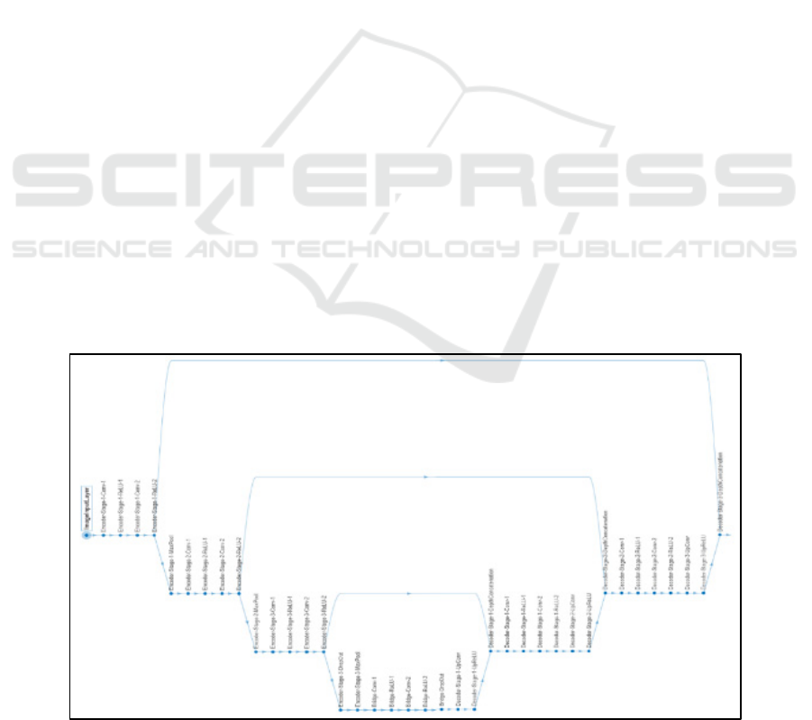
network’s model is based on the U-Net architecture
that implements a deep, pixel-wise regression. The
network’s architecture consists of two basic parts.
The first part is the encoder, which processes the
input image through a contraction path, where down-
sampling is being done by sequential convolutions,
ReLUs and max poolings. The second part is the
decoder, which processes the encoder’s result through
an expansion path, where up-sampling is performed
through sequential convolutions, ReLUs and
transposed convolutions. A main feature of this
architecture is its ability to find the right balance
between locality and context. Indeed, for better
localization accuracy, in every decoder’s step, skip
connections are being used, joining the outputs of the
transposed convolutions, with the feature maps from
the corresponding layer of the encoder part. Figure 4
visualizes the proposed network’s architecture.
Figure 4: U-net architecture of the proposed DCNN.
Buildings Extraction from Historical Topographic Maps via a Deep Convolution Neural Network
487
In the proposed DCNN, the goal is to predict, for
each pixel of the input patch, a value that is as close
as possible to the corresponding pixel value in the
ground truth patch. Regarding the objective function
employed to optimize the model the half-mean-
squared-error is applied, however not normalized by
the number of patch pixels, that is,
𝐶
1
2
𝑦
𝑦
(1)
where 𝐻,𝑊 denote the height and width of the
ground truth patch, 𝑦
is its binary pixel value and
𝑦
is the predicted response, given as output from the
DCNN. The above cost is backpropagated to all the
hidden layers of the DCNN and the network’s
parameters are updated iteratively using the Adam
optimizer (Kingma and Ba, 2014). Considering that
the output of the DCNN is a set of dense predictions,
where each pixel corresponds to a continuous
numerical value between 0 and 1, the output of the
network is converted to a binary one in order to be
compared to the corresponding ground-truth patch.
Training the U-Net is based on a large number of
images patches pairs extracted from the original and
the ground truth image, respectively. The original
image is a colored image map that depicts the
topographic area under consideration while the
ground truth is a binary image denoting only the
building footprints. A patch from the original image
is used as input to the network while the
corresponding binary ground truth image patch is
used as the desired network’s output. The patches are
created using three different approaches named
“Random”, “Grid-Random” and “Grid-Grid”,
respectively. They differ in the way the patches cover
the entire area of the original and ground truth
images.
In the “Random” case, patches from the original
and ground truth images are extracted in a fully
random fashion. The patch size is defined by the user
and is a system’s parameter. In order to avoid patch
overlapping the process keeps track of the patch
coordinates already created and allows new patches
whose coordinates differ from the previous ones by at
least a minimum number of pixels. Moreover, a cover
percentage parameter discards patches for which the
ground truth counterpart contains insufficient number
of active (black) pixels. This check ensures that the
ground truth generated patches contain an acceptable
minimum of valuable information, that is, pixels
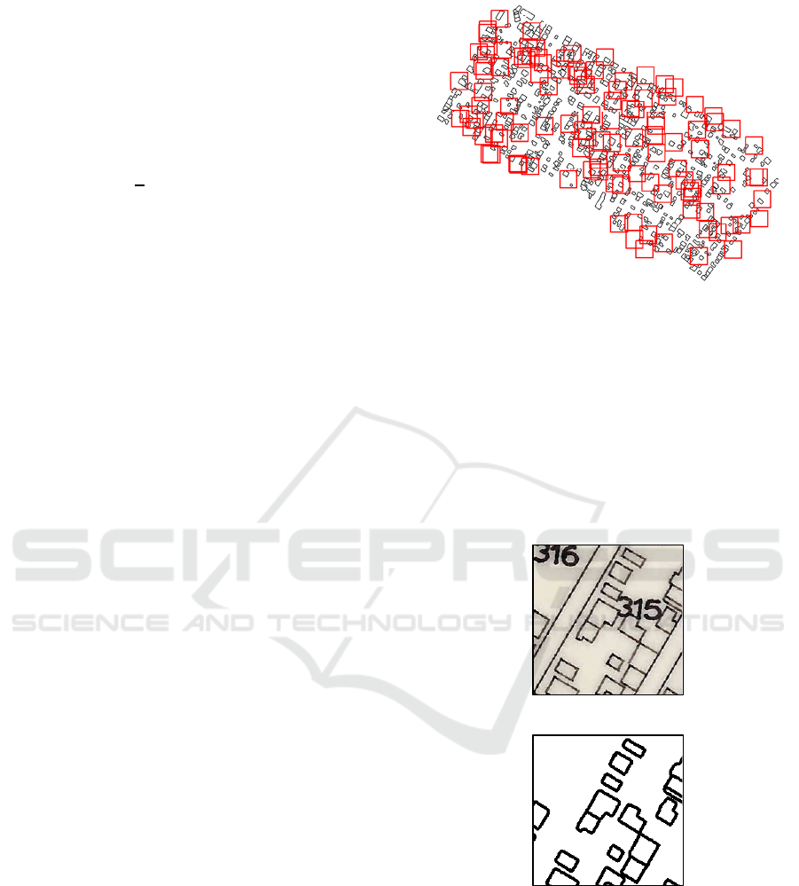
indicating building footprints. Figure 5 depicts an
instance of the “Random” patches’ creation process.
Figure 5: Snapshot of the “Random” patches process
implementation. The overall number of requested patches
is given by the user.
Identical patches coordinates apply to the original
color image and the ground truth image, respectively.
Figure 6 shows a pair of training patches. The patch
on the top is extracted from the original image and
serves as input for the DCNN network. The patch on
the bottom depicts the corresponding part of the
ground truth image which is used as the training target
of the network.
(
a
)
(
b
)
Figure 6: Example pair of training patches of size 224×224
pixels. (a) Patch in the original image (b) Corresponding
patch in the ground truth image.
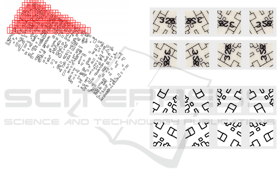
In the “Grid-Random” case, the patches from the
original and the ground truth images, are created in a
sequential sliding-window approach based on a user
defined grid step. Figure 7 depicts an example of the
process for patches of size 128×128 pixels. Again, a
VISAPP 2022 - 17th International Conference on Computer Vision Theory and Applications
488
cover percentage parameter prevents blank patches or
those with extremely few active pixels to be included.
While the patches are created in a sequential manner,
they are shuffled by re-indexing in a random order.
This sampling approach allows the DCNN to be
trained with patches that systematically cover, in a
grid fashion, the whole spatial range of the original
input and ground truth images while assuring a
certain percentage of patches diversity.
Finally, in case of the “Grid-Grid” sampling, the
patches are being extracted similarly to the “Grid-
Random” case, however the original sequential
indexing is preserved.
Figure 7: Snapshot of the “Grid-Random” and “Grid-Grid”
patches process implementation. The sequential patches
generation continues until the whole are is covered.
The last sampling approach affects the training
process since it does not allow the DCNN to be
trained with patches from the whole spatial range of
the original and ground truth images. Indeed, the
patches datasets are divided during the training of the
network into three parts: 50% of the dataset for
training, 25% for validation and 25% for testing. It is
important to notice that the splitting process is
sequentially performed based on the patches index.
Therefore, in the first two sampling scenarios
“Random” and “Grid-Random”, the patches
eventually cover the whole spatial range of the
original and ground truth images. In contrast, in the
third sampling case, “Grid-Grid”, only the first 50%
of the patches are used for training, leaving the next
25% and 25% for validation and testing, respectively.
Clearly, the minimum pixel difference parameter
for the “Random” sampling, the grid step parameter
for both the “Grid-Random” and “Grid-Grid”
sampling and the cover percentage parameter, for all
three cases, affect the total number of the extracted
patches pairs. Indeed, the lower the grid step or the
cover percentage value, the higher the number of
patches pairs that can be extracted. On the contrary,
increasing the minimum pixel difference between the
patches, decreases the number of extracted patches
pairs in the “Random” case.
After the patches are created, data augmentation
techniques are also involved in order to enhance the
size and quality of the training datasets facilitating the
network to build better models. Specifically, every
input and ground truth patch pair images are further
augmented by rotation by 90, 180, 270 degrees
in accordance with a horizontally flip leading to
an augmented set of 8 patches pairs, as shown in
Figure 8.
(a)
(
b
)
Figure 8: Data augmentation example for (a) an original
patch and (b) its corresponding ground truth instance. In
both rows, the first image is the original patch while the
following 7 patches are produced by the data augmentation
process.
3 EXPERIMENTAL RESULTS
The proposed method for extracting building
footprints from topographic map images is tested
under several experiment scenarios. The experiments
can be grouped into three different cases, according
to the sampling approach that has been followed. In
addition, for each sampling scenario three sub-
experiments were performed, using different patch
sizes.
Buildings Extraction from Historical Topographic Maps via a Deep Convolution Neural Network
489
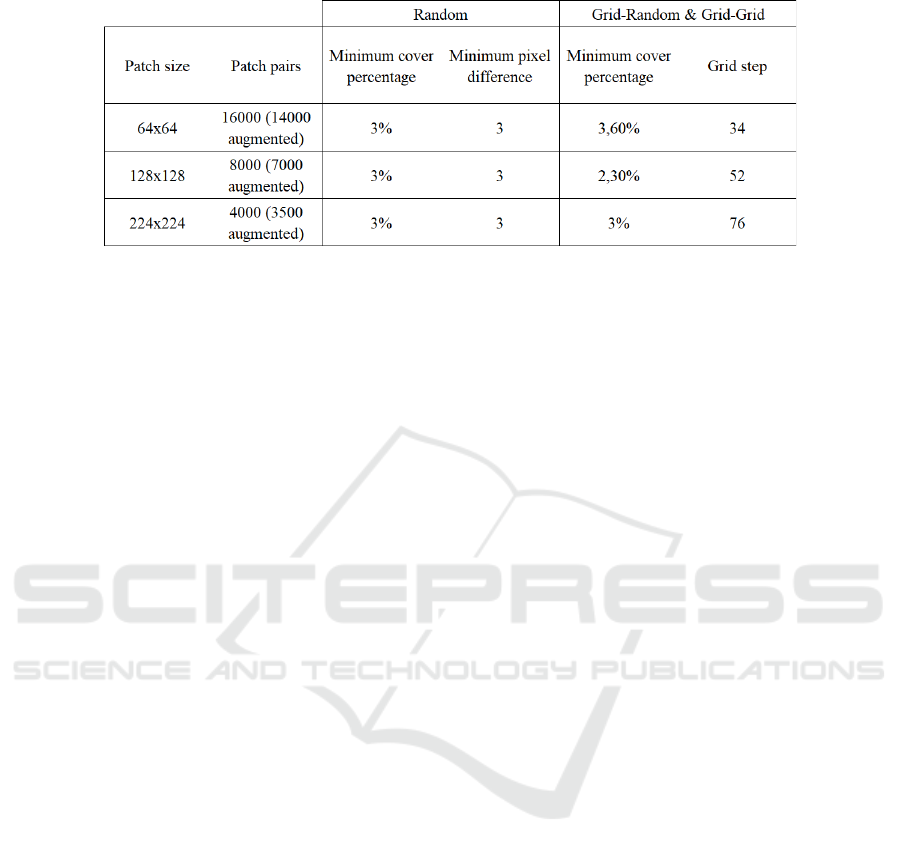
Table 1: Setup parameters used in the experiments.
Specifically, the first dataset contains 16000 input
and 16000 ground-truth patches of size 64×64 pixels
(the 2000 of them extracted from the original input
and ground-truth images, while the rest 14000 pairs
as a result of data augmentation), the second dataset
contains 8000 patches pairs of size 128×128 pixels
(accordingly, 1000 original and 7000 augmented) and
the third contains 4000 patches pairs of size 224×224
pixels (accordingly, 500 originally extracted and
3500 augmented). Table 1 summarizes the number of
patches as well as the parameter values for each
experiment dataset. Considering the DCNN, a
stochastic gradient descent approach is followed,
using Adam optimizer. The number of epochs is set
to 100, using a mini-batch of 8, with an initial learning
rate of 0.001, without learning rate scheduling.
Regarding the other network parameters, the default
values are applied as given in (Kingma and Ba, 2014).
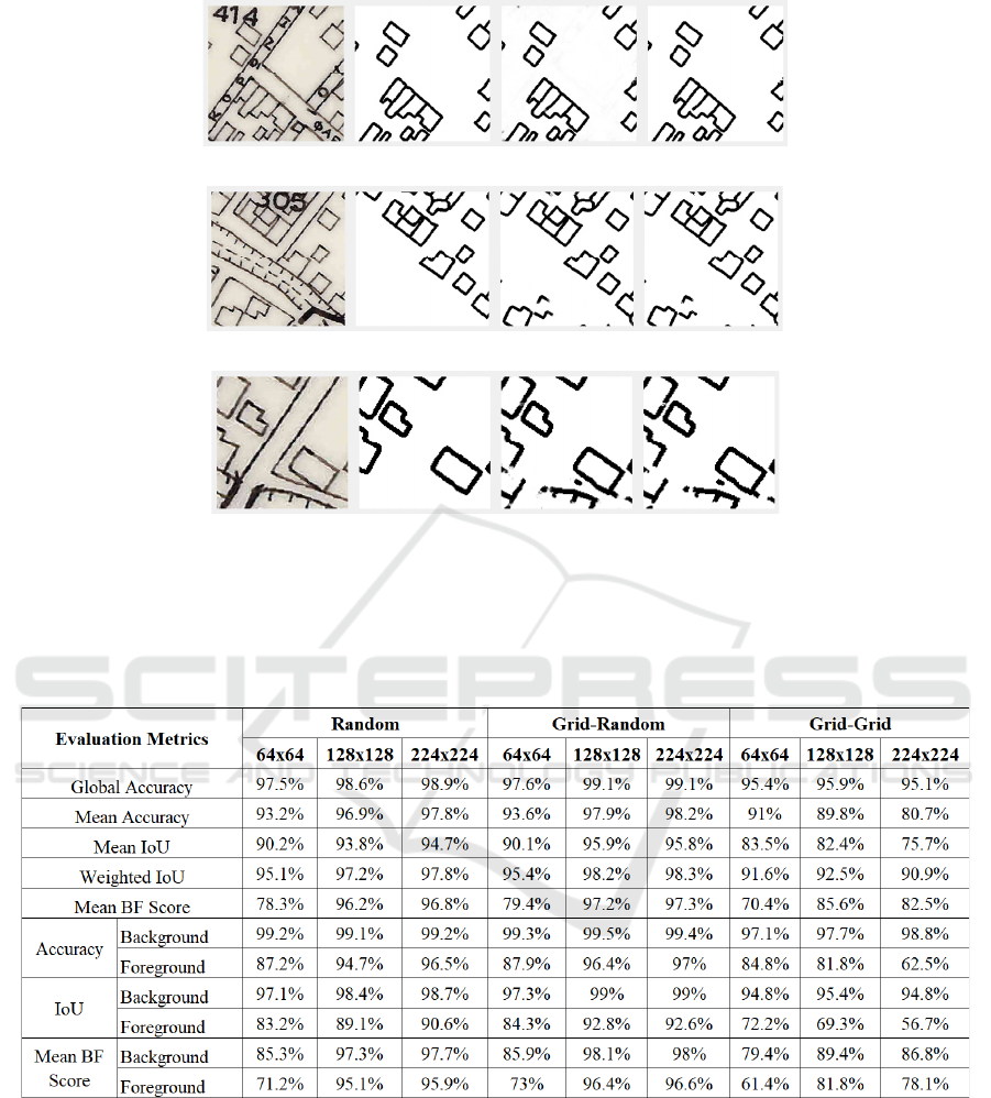
In Figure 9 three examples of networks predictions
are given. In each case, the first image is the input
patch from test data, the second image is the
corresponding ground-truth patch, the third image is
the network’s prediction and the fourth image is the
corresponding binarized predicted patch. Figure 9(a)
depicts a 224×224 “Grid-Random” sampling
example. It can be seen that the network efficiently
removed the building block number, the street lines
as well as the street names. Figure 9(b) demonstrates
a 224×224 “Random” sampling example where the
building block number is correctly removed even if it
overlaps several buildings. The graphical
representation of the riverbed is also ignored as object
of no interest. More interestingly, the buildings in the
lower left part are correctly detected by the network
even that they are missing from the ground truth.
Figure 9(c) refers to a 128×128 “Grid-Grid” sampling
example. The road lines are correctly ignored
however the network does not fully remove the river
graphics in the bottom left corner since similar
graphical content was not part of the training set.
The metrics used to evaluate the performance of
the DCNNs in the various experiments are based on a
pixel-by-pixel comparison between the ground truth
patch and the predicted binarized patch, counting the
true positives (TP), false positives (FP) and false
negatives (FN), respectively. For the ground truth
patches, as well as the predicted binarized images, the
white pixels are considered as the background class
while the black pixels denote the foreground class.
The metrics analytically are:
• Global Accuracy: The ratio of correctly
predicted pixels, regardless of class, to the
total pixels number of pixels.
• Mean Accuracy: The average accuracy of all
classes in all images, where for each class,
accuracy is the ratio of correctly classified
pixels to the total number of pixels in that
class, according to the ground truth, i.e.,
accuracy score = TP / (TP + FN).
• Mean Intersection over Union: The average IoU
score of all classes in all images, where for
each class, IoU is the ratio of correctly
classified pixels to the total number of ground
truth and predicted pixels in that class, i.e.,
IoU score = TP / (TP + FP + FN).
• Weighted Intersection over Union: The weighted
average IoU score of all classes in all images,
where for each class, weighted IoU is the
average IoU, weighted by the number of pixels
in that class.
• Mean Boundary F1 (BF) Score: The contour
matching score that indicates how well the
predicted boundary of each class aligns with
the true boundary. For the aggregate data set,
Mean BF Score is the average BF score of all
classes in all images and for each class, Mean
BF Score is the average BF score of that class
over all images.
VISAPP 2022 - 17th International Conference on Computer Vision Theory and Applications
490
(a)
(b)
(
c
)
Figure 9: Visual results of the proposed method. In each row the first image is the input patch from test data, the second image
depicts the corresponding ground-truth, the third image is the network’s prediction while the fourth image corresponds to the
binarized predicted patch (a) 224×224 “Grid-Random” example (b) 224×224 “Random” example (c) 128×128 “Grid-Grid”
example.
Table 2: Evaluation metrics results for the various experiments.
The results of the above metrics for all the
experimental scenarios are summarized in Table 2.
Regarding the class metrics, namely, Accuracy, IOU
and Mean BF Score, the most representative are the
ones that refer to the foreground class (black pixels)
since it contains the geographical features of interest,
i.e. the building footprints. It can be noticed that both
“Random” and “Grid-Random” sampling cases
increase their performance according to the patch size
which however is not the case in most of the “Grid-
Grid” cases. Moreover, the “Random” and “Grid-
Random” sampling cases provide high detection
accuracy, especially in the cases of 128×128 and
224×224 patches sizes. The sampling method
adopted in these two cases feeds the DCNN with
patches from multiple areas of the original image,
therefore providing the network with multiple
representations of desired input-output pairs. In the
Buildings Extraction from Historical Topographic Maps via a Deep Convolution Neural Network
491

case of “Grid-Grid” sampling, the DCNN is not that
high since it is trained with patches that do not cover
the whole spatial range of the original image. The best
global accuracy 99.1% is achieved for the “Grid-
Random” case for both patch sizes 128×128 and
224×224.
4 CONCLUSIONS
In this work a deep learning approach is presented
that tackles the problem of extracting buildings from
historical topographic maps. For this purpose, a
DCNN based on the U-Net architecture is trained in a
deep image-to-image regression mode. Experiments
on a historical topographic map demonstrate that the
proposed method efficiently extracts the buildings
from the map even when they are densely surrounded
or even overlapped by text or other geospatial
features. Evaluation under several sampling and patch
size scenarios gives promising results in terms of
building detection accuracy, especially when large
patch sizes are involved and when training the
network is based on randomly generated patches.
ACKNOWLEDGMENTS
Article processing charges are covered by the
University of West Attica.
REFERENCES
Dornaika, F., & Hammoudi, K. (2009, May). Extracting 3D
Polyhedral Building Models from Aerial Images Using
a Featureless and Direct Approach. In MVA (pp. 378-
381).
Fischer, A., Kolbe, T. H., Lang, F., Cremers, A. B.,
Förstner, W., Plümer, L., & Steinhage, V. (1998).
Extracting buildings from aerial images using
hierarchical aggregation in 2D and 3D. Computer
Vision and Image Understanding, 72(2), 185-203.
Hecht, R., Meinel, G., & Buchroithner, M. (2015).
Automatic identification of building types based on
topographic databases–a comparison of different data
sources. International Journal of Cartography, 1(1),
18-31.
Heitzler, M., & Hurni, L. (2020). Cartographic
reconstruction of building footprints from historical
maps: A study on the Swiss Siegfried map.
Transactions in GIS, 24(2), 442-461.
Kingma, D. P., & Ba, J. (2014). Adam: A method for
stochastic optimization. arXiv preprint
arXiv:1412.6980.
Laycock, S. D., Brown, P. G., Laycock, R. G., & Day, A.
M. (2011). Aligning archive maps and extracting
footprints for analysis of historic urban environments.
Computers & Graphics, 35(2), 242-249.
LeCun, Y., Bottou, L., Bengio, Y. & Haffner, P. (1998).
Gradient-based learning applied to document
recognition. Proceedings of the IEEE. 86(11): 2278 –
2324.
Li, B. H., Hou, B. C., Yu, W. T., Lu, X. B., & Yang, C. W.
(2017). Applications of artificial intelligence in
intelligent manufacturing: a review. Frontiers of
Information Technology & Electronic Engineering,
18(1), 86-96.
Peng, J., Zhang, D., & Liu, Y. (2005). An improved snake
model for building detection from urban aerial images.
Pattern Recognition Letters, 26(5), 587-595.
Ronneberger, O., Fischer, P., & Brox, T. (2015, October).
U-net: Convolutional networks for biomedical image
segmentation. In International Conference on Medical
image computing and computer-assisted intervention
(pp. 234-241). Springer, Cham.
Suzuki, S., & Chikatsu, H. (2003). Recreating the past city
model of historical town Kawagoe from antique map.
International Archives of Photogrammetry and Remote
Sensing, 34, 5.
Uhl, J. H., Leyk, S., Chiang, Y. Y., Duan, W., & Knoblock,
C. A. (2017, July). Extracting human settlement
footprint from historical topographic map series using
context-based machine learning. In 8th International
Conference of Pattern Recognition Systems (ICPRS
2017) (pp. 1-6).
Uhl, J. H., Leyk, S., Chiang, Y. Y., Duan, W., & Knoblock,
C. A. (2019). Automated extraction of human
settlement patterns from historical topographic map
series using weakly supervised convolutional neural
networks. IEEE Access, 8, 6978-6996.
Voulodimos, A., Doulamis, N., Doulamis, A., &
Protopapadakis, E. (2018). Deep learning for computer
vision: A brief review. Computational intelligence and
neuroscience, 2018.
VISAPP 2022 - 17th International Conference on Computer Vision Theory and Applications
492
