A Hierarchical Probabilistic Divergent Search

Applied to a Binary Classiﬁcation

Senthil Murugan

1 a

, Enrique Naredo

1 b

, Douglas Mota Dias

1,2 c

, Conor Ryan

1 d

Flaviano Godinez

3 e

and James Vincent Patten

1 f

University of Limerick, Limerick, Ireland

Rio de Janeiro State University, Rio de Janeiro, Brazil

Universidad Aut

onoma de Guerrero, Mexico

Keywords:

Genetic Programming, Novelty Search, Classiﬁcation.

Abstract:

The trend in recent years of the scientiﬁc community on solving a wide range of problems through Artiﬁcial

Intelligence has highlighted the beneﬁts of open-ended search algorithms. In this paper we apply a probabilis-

tic version for a divergent search algorithm in combination of a strategy to reduce the number of evaluations

and computational effort by gathering the population from a Genetic Programming algorithm into groups and

pruning the worst groups each certain number of generations. The combination proposed has shown encour-

aging results against a standard GP implementation on three binary classiﬁcation problems, where the time

taken to run an experiment is signiﬁcantly reduced to only 5% of the total time from the standard approach

while still maintaining, and indeed exceeding in the experimental results.

1 INTRODUCTION

Nowadays, the increasing interest of the scientiﬁc

community in the Artiﬁcial Intelligence and address-

ing a wide range of real-world problems has led to

increased interest in usage of open-ended search algo-

rithms as a means of ﬁnding novel solutions. One ex-

ample of an open-ended algorithm is Novelty Search

(NS) (Lehman and Stanley, 2008). According to (Pat-

tee and Sayama, 2019), there are many examples

throughout the history of evolution on Earth showing

that open-endedness is in fact a consequence of evo-

lution. An open-ended approach has the goal to learn

a repertoire of actions covering the whole space (Kim

et al., 2021).

The original version of NS utilises the k-NN al-

gorithm to explore the search space looking for novel

behaviors and requires an archive to save previous be-

haviors in order to avoid backtracking. Deﬁning the

right parameter k and managing the archive could rep-

https://orcid.org/0000-0003-0799-3079

https://orcid.org/0000-0001-9818-911X

https://orcid.org/0000-0002-1783-6352

https://orcid.org/0000-0002-7002-5815

https://orcid.org/0000-0001-5531-8989

https://orcid.org/0000-0002-1937-2774

resent a problem to efﬁciently implementing NS. One

approach to tackle these drawbacks is the Probabilis-

tic NS (Naredo et al., 2016), which is the method we

use in the work presented in this paper.

NS has been used successfully to address prob-

lems from different domains, such as the computa-

tional generation of video game content (Skjærseth

et al., 2021), on one of the most impactful tasks in

software development, namely bug repair (Trujillo

et al., 2021), and a multi-objective brain storm opti-

mization based on novelty search (MOBSO-NS) (XU

et al., 2021) as well as many others.

More recently a new family of algorithms called

quality-diversity algorithms (Pugh et al., 2016),

which combine behavior space exploration with a

global or local quality metric. An extensive study of

these related algorithms is however beyond the scope

of the research detailed in this paper.

The contributions of this paper are as follows: (i)

the introduction of an implementation of the prob-

abilistic version of novelty search (PNS) (Naredo

et al., 2016) using DEAP (Fortin et al., 2012) a is

a well known evolutionary computation framework,

and more speciﬁcally details of an implementation

that uses a Bernoulli distribution, (ii) the implemen-

tation of Pyramid Search (Ciesielski and Li, 2003) in

Murugan, S., Naredo, E., Dias, D., Ryan, C., Godinez, F. and Patten, J.

A Hierarchical Probabilistic Divergent Search Applied to a Binary Classiﬁcation.

DOI: 10.5220/0010841900003116

In Proceedings of the 14th International Conference on Agents and Artiﬁcial Intelligence (ICAART 2022) - Volume 2, pages 345-353

ISBN: 978-989-758-547-0; ISSN: 2184-433X

345

combination with OS and PNS, (iii) details of a case

study conducted on the performance of the implemen-

tation on three binary classiﬁcation problems, ranging

from easy to hard.

The remainder of this paper is organized as fol-

lows: In Section 2 a review of the main background

concepts. Next, Section 3 presents the experimental

set-up, outlining all of the considered variants and

performance measures. Section 4 presents and dis-

cusses the main experimental results of the described

research problem. Finally, Section 5 presents the con-

clusions and future work derived from this research.

2 BACKGROUND

2.1 Genetic Programming

Genetic Programming (GP) (Koza, 1992) is an evo-

lutionary algorithm which synthesize computer pro-

grams. The evolution process initiates with a popu-

lation of programs randomly created and assigning a

ﬁtness score according to the quality performance to

solve the problem.

This score is then used to select individual pro-

grams following the Darwinian principle of natural

selection to which genetic operators such as mutation

and crossover are later applied, which drives the evo-

lution of new programs in the hope that they are better

than their parents.

Traditionally, evolutionary algorithms such as GP

guide the search by rewarding individuals close to the

predeﬁned optimal ﬁtness score target, which we re-

fer to in this work as Objective-based search or for

short OS. For instance, a predeﬁned score target for

a binary classiﬁcation problem is is to get 100% of

classiﬁcation rate.

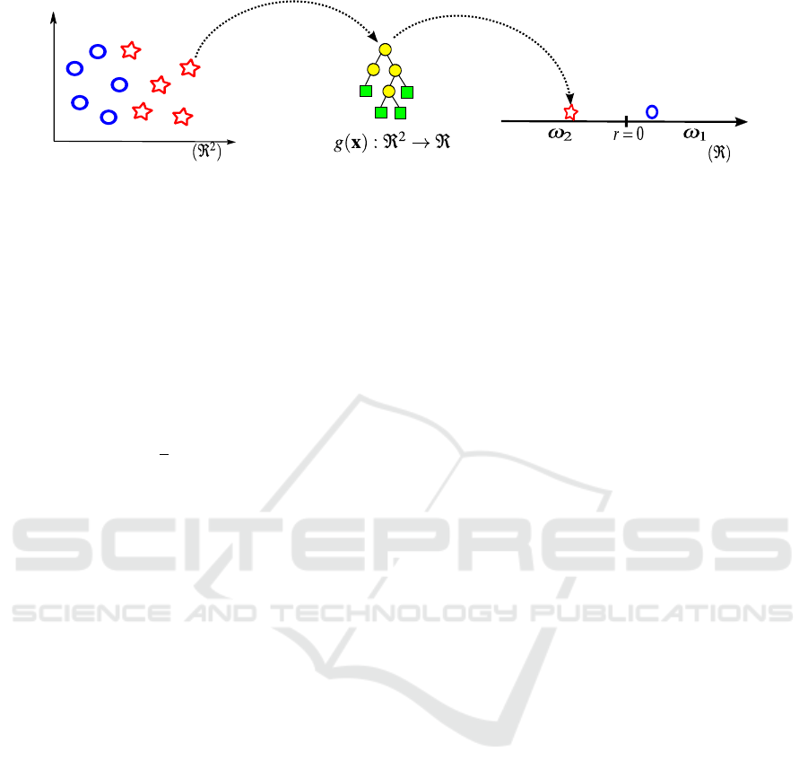
In this work, we use binary classiﬁcation problems

and apply the Static Range Selection (SRS) described

by Zhang and Smart (Zhang and Smart, 2006). A de-

piction of the SRS based classiﬁcation can be found

in ﬁgure 1. In this method, the goal is to evolve a

function g : ℜ

→ ℜ represented in the ﬁgure as a

tree, which can map the vector of samples x from the

hyper-dimensional feature space into a 1-dimensional

space. In the ﬁgure for visualizing purposes we use

a 2D feature space (d

), meaning that each x

), and the general case is x

= (d

,...,d

For a binary classiﬁcation problem a typical

threshold to use is zero to split in a natural way the

one-dimensional space into two regions, where we

have at the right the region ω

with positive num-

bers and at the left the region ω

with negative num-

bers. Predictions from the GP-classiﬁers are in these

regions, where

y are the predictions to the true class

y ∈ {0,1}. More speciﬁcally, for the binary case, we

have as predictions a vector of 0s and 1s;

y = [

= 1,...,

= 0], for short

y = [0,1,...,0].

The performance of a GP-classiﬁer is measured

comparing the predictions

y against the true class

y assigning 1 when the sample classiﬁcation is cor-

rect and 0 otherwise, resulting in a vector b =

,...,b

], where the 1s are successes or hits, then

the accuracy of a GP-classiﬁer is computed as follows

Accuracy =

hits

number of samples

∑

b = 1

|b|

, (1)

where accuracy gives us an aggregated information of

each GP-classiﬁer through a single score value.

2.2 Novelty Search

Novelty search (NS) (Lehman and Stanley, 2008) is a

diversity mechanism with a high search efﬁciency that

helps the search to escape from local optima avoiding

premature convergence.

NS is an alternative to OS, in which the objec-

tive function is replaced by a measurement of novelty

and uniqueness (Lehman and Stanley, 2010). On one

hand, we have OS rewarding individuals close to the

target and on the other hand we have NS rewarding

the most novel individuals. NS uses a behavior de-

scriptor, which must capture the actions taken by the

individual to make progress in the solution space. For

a binary classiﬁcation problem one feasible behavior

descriptor is b described in the previous section 2.1,

whereas OS uses a score value, described in the Equa-

tion 1, where the higher score the better. Therefore,

gradients in OS are towards objective, whereas the NS

is towards behaviour.

The original measure of novelty (Lehman and

Stanley, 2008) uses the k-nearest neighbors algorithm

(k-NN), but instead of concern as to the compactness

of the cluster where the individual is located, NS mea-

sures the sparseness S around each behavior b

. In

other words, NS measures how different is the behav-

ior from one individual against the behavior of its k-

neighbors from b

, by computing the following equa-

tion:

S(b

) =

∑

l=1

dist(b

) , (2)

where b

is the lth-nearest from k-neighbours re-

spect to the average metric dist, which is a domain-

dependent measure of the behavioural descriptor. A

general interpretation of this measure is that a behav-

ior b is novel when located in a sparse region, but not

ICAART 2022 - 14th International Conference on Agents and Artiﬁcial Intelligence

346

Feature space

1-dimensional space

Figure 1: Graphical depiction of SRS-GPC.

novel when located in a dense region. This NS version

is easy to implement, but requires the deﬁnition of k

and this is computationally intensive for large training

sets.

In order to avoid backtracking, the revisiting of

regions that were previously explored in the search

space, NS needs to save behaviors to an archive from

the current generation. The behaviors from the cur-

rent generation and from the archive can form a bigger

seta of behaviors to compute sparseness S as follows:

S(b) =

∑

l=1

dist(b

) , (3)

where a

is the lth-nearest from k-neighbours behav-

iors from both the actual generation t and the archive

with behaviors from the previous generation t-1. For

this version, when dealing with easy problems the

amount of behaviors is usually manageable, but with

more complicated problems a more considered man-

agement strategy is required. A well known method

to manage the behaviors as a queue is the ﬁrst-in ﬁrst-

out (FIFO). In this paper, we are not using the original

version of NS.

2.3 Probabilistic Novelty Search

The original version of NS requires the tuning the pa-

rameter k, to decide what behaviors to store in the

archive and to manage the archive. Probabilistic Nov-

elty Search (PNS) (Naredo et al., 2016) aims to tackle

these drawbacks, eliminating the parameter k, not us-

ing any archive, and as a consequence considerably

reducing the computational effort without compro-

mising the quality performance.

PNS is a probabilistic approach towards comput-

ing novelty using the same behavioral descriptor b for

NS. PNS assumes that a behaviour b

from an individ-

ual is independent of the behavior from any other in-

dividual, modeling the behaviors as random vectors.

During the evolutionary search process, performed by

GP, we have a population of B behaviors correspond-

ing to the GP-classiﬁers,

= [b]

[b]

,[b]

,...,[b]

, (4)

where j is the index for each individual in the popu-

lation, and t is the actual generation. Expanding the

mathematical notation we have a matrix of behaviors

each generation, as follows







1,1

··· ··· b

1,n

i, j

m,1

··· ··· b

m,n







. (5)

Since we are using the hits, the matrix contains 0s

and 1s. If we consider each outcome from the behav-

ior descriptor as a random variable R, we can model

the behaviors using a Bernoulli distribution, where

the random variable R takes the success value 1 with

probability p, and the failure value 0 with probability

q = 1 − p. Then, the probability of success is given

by P(R = 1) = p, and the probability of failure by

P(R = 0) = q = 1 − p, where p and q depends on the

number of samples and it is a well known fact that the

estimator of p is the sample mean.

Taking the successful case where the random vari-

able R = 1, we consider the hit from each behavior

descriptor b

i, j

= 1, in order to reduce the complexity

of the mathematical notation and get a more readable

notation, we simplify it by removing t, assuming that

each behavior from the population is from the actual

generation t.

As an illustrative example, say we had 7 samples

from the dataset (rows) and 6 individuals (columns)

in the population, then the order of the matrix B

∗

7 × 6. As can be seen in the matrix B shown in the

Equation 6, in the ﬁrst row it has all 0s, and in the

last row has all 1s, meaning that the ﬁrst is difﬁcult

to classify, whereas the last one is an easy sample to

classify.

A Hierarchical Probabilistic Divergent Search Applied to a Binary Classiﬁcation

347

B =







0 0 0 0 0 0

0 0 0 1 0 0

0 1 1 0 0 1

1 0 1 1 1 0

0 1 1 0 0 0

1 0 0 1 1 1

1 1 1 1 1 1







, p =













. (6)

The probability p for each sample shown in B to be

correctly classiﬁed is given by the rate of number of

successes R = 1 over the number of observations and

shown in the vector p. For instance, the ﬁrst sample

has a probability of

/6 = 0, while the last one has

/6 = 1 with 100% of successes.

We consider the product of the hit matrix, B with

its probability of hits, p. To make the product pos-

sible, the vector is converted to a diagonal matrix

D = diag(p), where each diagonal component is p

This way the product is P

= DB, where it only con-

siders the hits cases, as follows:







0 0 0 0 0 0

0 0 0

/6 0 0

/6 0

/6 0 0 0

/6 0 0







, (7)

for the ﬁrst individual we have [0,0,0,

/6,0,

/6,

/6]

and summing up these probabilities we have

/6 =

2.33. Doing similar computation for the rest of

the individuals results in a vector of accumulated

expected values [2.33,1.83,2.50,2.50,2.33,2.17] re-

lated to each individual.

The case where all the individuals successfully

classify each sample 6/6 = 1 and having 7 samples in

this example, then the maximum accumulated prob-

ability is 7, normalizing the previous vector we have

[0.33,0.26,0.35,0.35,0.33,0.31]. Finally, we have an

aggregated probability information where PNS cap-

tures the probability differences among the individu-

als’ behaviors.

PNS(b)

∑

i=1

i, j

) + ε

, (8)

where ε is the total error of the probabilistic model

against the true model. The novelty of each individ-

ual behavior is inversely proportional to the probabil-

ity of predicting correctly (hit) each sample. Instead

of managing an archive, we can save the parameters

from the probability density function (PDF) for each

sample and update them by using for example a con-

volution strategy between the previous and the actual

PDFs.

2.4 Pyramid Search

There is a wide range of approaches in the literature

to address evolutionary algorithms in a hierarchical

way. For instance, a recent approach to address Deep

Learning is proposed in (Houreh. et al., 2021), where

the authors addresses the problem of evolving a neu-

ral network in a hierarchical way using GA as the

search engine to automatically ﬁnd the best architec-

ture combination from a set of U-net architectures to

solve the Retinal Blood Vessel Segmentation.

A novel hierarchical approach named Pyramid is

proposed by (Ryan et al., 2020), where the main idea

is to decompose a complex problem into subsets of

simpler versions from the original and while scaling

up to ﬁnally address the entire problem the popula-

tion size is reduced keeping only the top individuals

in each step.

Another hierarchical approach which shares part

of the name with the previous approach is the Pyra-

mid Search proposed by (Ciesielski and Li, 2003).

In this approach the strategy is to split the popula-

tion into groups and prune them a certain number of

generations to reduce the number of evaluations and

keeping competitive results. In this work, we use the

latter approach applying it to solve a set of classiﬁca-

tion problems.

According to (Ciesielski and Li, 2003), Pyramid

Search evolve optimal solutions using a reduced num-

ber of generations and individuals in the population

by removing the worst performing groups. The Algo-

rithm 1 gives the guidelines for the implementation of

this method.

Algorithm 1: Pyramid Search.

Input: The given problem and the solution representation.

Output: Best solution (with less groups of individuals).

1 Pop size = No. of individuals in a group

2 Groups = No. of groups

3 Pruning ratio = No. of least ﬁt groups to be removed

4 Gens to prone = No. of generation to be pruned

5 Initialize groups = Individuals(Pop size)

6 while problem not solved or single group remains: do

7 Do evolution process

8 Prune Groups(pruning ratio * groups)

9 if problem not solved then

10 Continue iterations until single population exists

11 else

12 Problem solved or max generations is reached

In this approach the evolutionary process starts in

the traditional manner by randomly creating an initial

population, but in the next step, Pyramid Search splits

the population into groups of ﬁxed size. Each group

is ranked based on its top individual, in other words,

ICAART 2022 - 14th International Conference on Agents and Artiﬁcial Intelligence

348

the best individual from each group gives the repre-

sentative ﬁtness score to rank the group. The prun-

ing process is based on the pruning ratio parameter,

where the groups showing the lowest ﬁtness value will

be discarded, in other words, the groups bring their

champions and the worst of them are executed with

the whole group (all of them). The rest of the cham-

pions go to the next level with their entire group, this

pruning process continue until the problem is solved

or the maximum number of generations are reached.

Figure 2: Graphical depiction of Pyramid Search.

In the ﬁgure 2, we can see a visual representa-

tion of the pruning process in the Pyramid Search. In

the example every ﬁve generations a group competi-

tion takes place and the worst two groups are removed

(represented by a red cross), an alternate way of look-

ing at this is that the groups are sorted in such a way

that the worst are placed at the ends. At the generation

20, only one group is removed and it remains until the

evolutionary process stop.

3 EXPERIMENTAL SETUP

We designed a set of experiments based on binary

classiﬁcation problems to test both methods OS and

PNS, and their combination with Pyramid, namely

Py-OS and Py-PNS, particularly for the PNS meth-

ods we neither use an archive nor updated the PDF

with previous distributions parameters.

3.1 Datasets

Three datasets were selected: Cervical Cancer, Heart

Disease, and Genetic Variation, sorted, from easy to

hard.

Dataset 1: Cervical Cancer. The dataset (Repos-

itory, a) contains features such as age sex, smoke

Table 1: Binary Classiﬁcation Datasets.

Datasets Class Vars Samples

Cervical Cancer

2 33 857

Heart Disease

†

2 31 303

Genetic Variation

2 57 3373

habits, STDs & other hormonal reading & the depen-

dent variable represents the predictions of indicators

or diagnosis of cervical cancer (Classes 0 or 1).

Dataset 2: Heart Disease. The dataset (Repository,

b) has 13 independent variables which represents at-

tributes such as age, sex, serum cholesterol, chest pain

types, heart rate etc. The dependent variable refers

to the presence of heart disease in the patient. Class

0 represents no/less chance of heart attack, and the

Class 1 represents more chance of heart attack.

Dataset 3: Genetic Variation Classiﬁcation. This

is a public dataset containing annotations about hu-

man genetic variants (Clinvar, ). These variants are

manually classiﬁed by clinical laboratories on a cat-

egorical spectrum ranging from benign, likely be-

nign, uncertain signiﬁcance, likely pathogenic, and

pathogenic. Variants that have conﬂicting classiﬁ-

cations can cause confusion when clinicians or re-

searchers try to interpret whether the variant has an

impact on the disease of a given patient. The objec-

tive is to predict whether a Clinical Var variant will

have conﬂicting classiﬁcations. This is presented here

as a binary classiﬁcation problem, where each record

in the dataset is a genetic variant.

3.2 GP Parameters

Table 2 shows the parameters for GP in the top section

and for the Pyramid Search at the bottom. The ﬁtness

function is the accuracy as shown in the Equation 1.

Finally, all experiments were conducted using DEAP

(Fortin et al., 2012).

4 EXPERIMENTAL RESULTS

The table 3 summarizes the experimental results, con-

ducted over 30 experimental runs. The ﬁrst column

shows the datasets: Cervial Cancer, Heart Disease,

and Genetic Variation, where the ﬁrst is the easiest

and the last the hardest. Second column shows the

methods used: OS, PNS, Py-OS, Py-PNS, where OS

stands for the Objective-based search and it is the tra-

ditional approach to rewards solutions closer to the

target. The second method is PNS, which stands for

A Hierarchical Probabilistic Divergent Search Applied to a Binary Classiﬁcation

349

Table 2: GP and Pyramid Search parameters.

Parameter Value

Runs 30

Population 200

Replacement Tournament

Crossover 0.7

Function Set I +, -, *, /, cos, sin

Function Set II log, and, or ,not, if

Pyramid Search

Pruning Ratio 0.2

Prune After Generations 5

No.of.Groups 10

Group Size 20

Probabilistic Novelty Search, which is a probabilis-

tic approach to implement a divergent search. The

rest are combinations of the ﬁrst two methods with

the Pyramid Search.

The experimental results start with the column

’Train’, which stands for the average results in all runs

using the training dataset, and ’Test’ for the he aver-

age results on test dataset. The column with ’Time;

give us the information of the time spent by each run

in average. Finally, the ’AvgSize’ stands for the av-

erage size of the solutions considering the number of

nodes in the GP-tree.

4.1 Results in Training

Results shown in table 3, speciﬁcally for the Cervical

Cancer dataset in training favors OS but does not have

a statistical signiﬁcant difference from PNS, even the

standard deviation are similar among them. On the

other hand, the combination using Pyramid Search

shows results which are inferior to OS and PNS, but

still in the same order, so both combinations show

very good results. The results show PNS performs

better in training for the Heart Disease with a signiﬁ-

cant difference against OS. The results in training for

the Genetic Variation dataset, again place PNS as the

champion, but followed closely by OS and the Pyra-

mid combination are not that far.

ﬁgure 3 shows the convergence plot for the three

datasets using OS and PNS, where it can be noted

that the degree of difﬁculty for the methods to evolve

good solutions for each of the datasets, the results

clearly show that in training the easiest dataset is Cer-

vical Cancer while the hardest is the Genetic Varia-

tion dataset. Figure 4 shows the convergence from the

combination with Pyramid. Cervical Cancer dataset

OS shows a better convergence can be seen and PNS

struggles to continue evolving solutions. In the rest of

the datasets while Py-OS demonstrates a tendency to

evolve good solutions, they are not as good as those

evolved by OS and PNS, with Py-PSN getting trapped

at a local optima in both datasets. A summarised per-

formance in training is shown in the Figure 5, where

Py-OS is worst than OS and PNS, and Py-PNS can-

not ﬁnd good solutions in training as the rest of the

methods.

4.2 Results in Test

Results in test shown for Cervical Cancer in table 3

interestingly favor Py-PNS, which shows the worst

performance in training. Morover, Py-PNS is the

champion in test on all the datasets, this conﬁrm the

hypothesis that PNS can ﬁnd novel solutions and in

combination with Pyramid Search keeps best solu-

tions with a reduced number of individuals from the

original population.

The ﬁgure 6 shows the boxplots of the perfor-

mance of each method in test, it can be observed in

these that the median of Py-PSN is always above than

the rest of the methods tested.

4.3 Time Consumption

The experimental results shown in the table 3 regard-

ing the time taken in average to run a single experi-

ment from each method place Py-OS in the ﬁrst place

in all the datasets followed close by Py-PNS, inter-

estingly PNS goes third in Cervical Cancer, but got

the last position on the remaining datasets. This same

trend is graphically observed in the Figure 7, where

clearly both combinations using Pyramid in average

take 5% of the time used by OS or PNS.

4.4 Average Size

The experimental results shown in the table 3 re-

garding the average size from each method place Py-

PNS in the ﬁrst place followed by Py-OS, interest-

ingly PNS ranks third in Cervical Cancer, but got the

last place on the remaining datasets. The ﬁgure 8

shows the size grow for OS and PNS. For Cervical

Cancer OS shows higher size in average than PNS,

even though around the generation 85 both method

show similar size average. For Heart Disease and

Genetic Variation, OS shows a more ﬂat grow rate,

whereas PNS evolves more complex solutions on av-

erage. PNS does not get better performance than OS,

but observing the boxplots from ﬁgure 6 can be ob-

served that PNS gets a more diverse set of solutions

than OS. The trend observed in the ﬁgure 9 regarding

the average size of the solutions evolved by the meth-

ods in combination with Pyramid shows that Py-PNS

evolve smaller solutions than Py-OS.

ICAART 2022 - 14th International Conference on Agents and Artiﬁcial Intelligence

350

Table 3: Experimental results averaged over 30 runs, best results are bold.

Dataset Method Train Test Time Avg Size

Cervical Cancer OS 0.9620 ±0.003 0.9580 ±0.002 98.92 ±0.00 5.00 ±8.68

Py-OS 0.9609 ±0.001 0.9582 ±0.002 5.82 ±0.00 4.71 ±0.51

PNS 0.9619 ±0.003 0.9583 ±0.003 125.56 ±0.00 4.25 ±3.86

Py-PNS 0.9575 ±0.004 0.9621 ±0.006 6.52 ±0.00 3.44 ±0.37

Heart Disease OS 0.8221 ±0.019 0.7289 ±0.059 29.65 ±0.00 5.69 ±3.44

Py-OS 0.7952 ±0.020 0.7194 ±0.046 1.86 ±0.00 6.13 ±1.93

PNS 0.8272 ±0.021 0.7322 ±0.053 38.31 ±0.00 7.48 ±5.31

Py-PNS 0.7588 ±0.010 0.7362 ±0.044 2.25 ±0.00 3.13 ±0.29

Genetic Variation OS 0.7479 ±0.001 0.7222 ±0.001 411.30 ±0.00 9.17 ±6.22

Py-OS 0.7472 ±0.000 0.7222 ±0.002 25.36 ±0.00 6.80 ±2.41

PNS 0.7488 ±0.001 0.7224 ±0.002 533.92 ±0.00 13.01 ±14.34

Py-PNS 0.7458 ±0.000 0.7243 ±0.000 25.60 ±0.00 2.82 ±0.30

REFERENCES

Ciesielski, V. and Li, X. (2003). Pyramid search: finding
solutions for deceptive problems quickly in genetic
programming. In The 2003 Congress on Evolution-
ary Computation, 2003. CEC ’03., volume 2, pages
936–943 Vol.2.
Clinvar, N. Genetic variant classification dataset.
ftp://ftp.ncbi.nlm.nih.gov/pub/clinvar/vcf\ GRCh37/
clinvar.vcf.gz. Online; accessed 28-September-2021.
Fortin, F.-A., De Rainville, F.-M., Gardner, M.-A., Parizeau,
M., and Gagn
´
e, C. (2012). DEAP: Evolutionary algo-
rithms made easy. Journal of Machine Learning Re-
search, 13:2171–2175.
Houreh., Y., Mahdinejad., M., Naredo., E., Dias., D., and
Ryan., C. (2021). Hnas: Hyper neural architecture
search for image segmentation. In Proceedings of the
13th International Conference on Agents and Artifi-
cial Intelligence - Volume 2: ICAART,, pages 246–
256. INSTICC, SciTePress.
Kim, S., Coninx, A., and Doncieux, S. (2021). From explo-
ration to control: Learning object manipulation skills
through novelty search and local adaptation. Robotics
and Autonomous Systems, 136:103710.
Koza, J. R. (1992). Genetic Programming - On the pro-
gramming of Computers by Means of Natural Selec-
tion. Complex adaptive systems. MIT Press.
Lehman, J. and Stanley, K. (2008). Exploiting open-
endedness to solve problems through the search for
novelty. In Bullock, S., Noble, J., Watson, R., and Be-
dau, M. A., editors, Artificial Life XI: Proceedings of
the Eleventh International Conference on the Simula-
tion and Synthesis of Living Systems, pages 329–336.
MIT Press, Cambridge, MA.
Lehman, J. and Stanley, K. O. (2010). Efficiently evolving
programs through the search for novelty. In Pelikan,
M. and Branke, J., editors, GECCO, pages 837–844.
ACM.
Naredo, E., Trujillo, L., Legrand, P., Silva, S., and Mu
˜
noz,
L. (2016). Evolving genetic programming classifiers
with novelty search. Information Sciences, 369:347 –
367.
Pattee, H. H. and Sayama, H. (2019). Evolved Open-
Endedness, Not Open-Ended Evolution. Artificial
Life, 25(1):4–8.
Pugh, J. K., Soros, L. B., and Stanley, K. O. (2016). An
extended study of quality diversity algorithms. In
Proceedings of the 2016 on Genetic and Evolution-
ary Computation Conference Companion, GECCO
’16 Companion, page 19–20, New York, NY, USA.
Association for Computing Machinery.
Repository, U. M. L. Cervical cancer dataset.
https://archive.ics.uci.edu/ml/datasets/Cervical+
cancer+\%28Risk+Factors\%29. Online; accessed
28-September-2021.
Repository, U. M. L. Heart disease dataset. https://
archive.ics.uci.edu/ml/datasets/heart+disease. Online;
accessed 28-September-2021.
Ryan, C., Rafiq, A., and Naredo, E. (2020). Pyramid: A
hierarchical approach to scaling down population size
in genetic algorithms. pages 1–8.
Skjærseth, E. H., Vinje, H., and Mengshoel, O. J. (2021).
Novelty search for evolving interesting character me-
chanics for a two-player video game. In Proceedings
of the Genetic and Evolutionary Computation Confer-
ence Companion, GECCO ’21, page 321–322, New
York, NY, USA. Association for Computing Machin-
ery.
Trujillo, L., Villanueva, O. M., and Hernandez, D. E.
(2021). A novel approach for search-based program
repair. IEEE Software, 38(4):36–42.
XU, Q., Pan, X., Wang, J., Wei, M., and Li, H. (2021).
Multiobjective brain storm optimization community
detection method based on novelty search. Hindawi,
Mathematical Problems in Engineering, 2021:14. Ar-
ticle ID 5535881.
Zhang, M. and Smart, W. (2006). Using gaussian distri-
bution to construct fitness functions in genetic pro-
gramming for multiclass object classification. Pattern
Recogn. Lett., 27(11):1266–1274.