
Explainable Clustering Applied to the Definition of Terrestrial Biomes
Mohamed Redha Sidoumou
1 a
, Alisa Kim
2
, Jeremy Walton
3 b
, Douglas I. Kelley
4 c
,
Robert J. Parker
5 d
and Ranjini Swaminathan
6 e
1
Amazon Web Services, U.K.
2
Amazon Web Services, Germany
3
Met Office Hadley Centre for Climate Science and Services, Exeter, U.K.
4
U.K. Centre for Ecology and Hydrology, Wallingford, U.K.
5
National Centre for Earth Observation, Space Park Leicester, University of Leicester, U.K.
6
National Centre for Earth Observation, Department of Meteorology, University of Reading, U.K.
Keywords:
Explainable AI, Explainability, Biomes, Clustering, Segmentation.
Abstract:
We present an explainable clustering approach for use with 3D tensor data and use it to define terrestrial
biomes from observations in an automatic, data-driven fashion. Our approach allows us to use a larger number
of features than is feasible for current empirical methods for defining biomes, which typically rely on expert
knowledge and are inherently more subjective than our approach. The data consists of 2D maps of geophysical
observation variables, which are rescaled and stacked to form a 3D tensor. We adapt an image segmentation
algorithm to divide the tensor into homogeneous regions before partitioning the data using the k-means algo-
rithm. We add explainability to the classification by approximating the clusters with a compact decision tree
whose size is limited. Preliminary results show that, with a few exceptions, each cluster represents a biome
which can be defined with a single decision rule.
1 INTRODUCTION
Natural environment data are complex, noisy and
challenging to analyse. However, interesting
results—see, for example (Ben-Dor et al., 1999)—
can be obtained by the application of data cluster-
ing, which aims to group similar data points accord-
ing to some chosen measure. Clustering is an ex-
ample of unsupervised learning, in which algorithms
find structures and relationships in the data without
making use of labels applied to the data, or with any
preconceptions of patterns in the data. Many cluster-
ing algorithms have been developed such as k-means
(Hartigan and Wong, 1979) and hierarchical clus-
tering (Johnson, 1967). However, before computa-
tional clustering methods existed, experts used empir-
ical methods to categorise their data, relying on their
a
https://orcid.org/0000-0001-6021-0737
b
https://orcid.org/0000-0001-7372-178X
c
https://orcid.org/0000-0003-1413-4969
d
https://orcid.org/0000-0002-0801-0831
e
https://orcid.org/0000-0001-5853-2673
domain-specific knowledge and expertise.
Terrestrial biomes are constructs that cluster to-
gether similar geographical areas. More specifically,
a biome is defined as a community of plants with sim-
ilar functions which form in response to a shared cli-
mate. Examples of biomes include grassland, tropi-
cal rainforest and desert. Biome distributions affect
life on Earth and represent helpful constructs for the
organization of knowledge about ecosystems. Clus-
tering is a natural choice for the characterization of
biomes. Experts have used empirical approaches us-
ing data derived from precipitation and temperature to
make such constructs, leading to the K
¨
oppen-Geiger
(KG) tree model (Peel et al., 2007), built using rules
to decompose the terrestrial map into distinct biomes.
These methods rely on expert assessment and inter-
pretation of observational data to assess future envi-
ronmental change. While this has led to a plethora
of biome representations, very few of these biome
maps target the comparatively coarser scale vegeta-
tion cover changes that are associated with numerical
Dynamic Global Vegetation Models (DGVMs) and
586
Sidoumou, M., Kim, A., Walton, J., Kelley, D., Parker, R. and Swaminathan, R.
Explainable Clustering Applied to the Definition of Terrestrial Biomes.
DOI: 10.5220/0010842400003122
In Proceedings of the 11th International Conference on Pattern Recognition Applications and Methods (ICPRAM 2022), pages 586-595
ISBN: 978-989-758-549-4; ISSN: 2184-4313
Copyright
c
2022 by SCITEPRESS – Science and Technology Publications, Lda. All rights reserved

the climate models which incorporate them. Mod-
elling studies are often forced to re-interpret biome
maps designed for very different ecological purposes.
In addition, the specific motivation for an ecological
study can affect which variables are selected, causing
this to be less objective.
An alternative approach is to use expert-led deci-
sions to partition a small number of bioclimatic vari-
ables into biomes (Prentice et al., 2011; Sato et al.,
2021). While these are custom-made for climate
model resolutions, they are restricted to a small num-
ber of variables—for example, (Prentice et al., 2011)
uses between two and five variables, depending on the
biome of interest—due to limits on the number of fea-
tures which can be assessed by human experts. Biome
definitions can also cut across areas of dense biocli-
mate space, suggesting biome boundaries and expert
assessment for biome definitions do not necessarily
align.
Despite their shortcomings, these empirical ap-
proaches have the merit of being interpretable—that
is, the reasons for the classification of each biome can
be understood. Whilst interpretability is not manda-
tory to validate and use a particular clustering method,
it is a feature which appeals to experts, offering a way
to understand the results and learn from the findings.
For this reason, we seek a clustering methodology
with an application to terrestrial biomes which, in ad-
dition to being objective, automatic and data-driven,
is also interpretable.
2 RELATED WORK
The biome map of Olson and his colleagues (Olson
et al., 2001) is perhaps the most commonly used in
DGVMs—e.g., (Sellar et al., 2019; Forrest et al.,
2020). This is a meta-analysis of previously pub-
lished ecosystem maps which have been grouped
into biomes in consultation with regional experts and
global ecologists. The map, commissioned by the
World Wide Fund for Nature, is designed specifically
for the global coordination of regional and local con-
servation efforts—a very different purpose to global
land surface model evaluation. The Olson biome
map provides more detail than can be represented by
DGVMs or climate models, and as a result, global
vegetation studies have aggregated Olson biomes (in
a fashion which is largely inconsistent).
The KG tree model is more targeted to global
biome distributions, and has been considered as the
standard method for biome classification (Kottek
et al., 2006). KG uses temperature and precipitation
measurements with decisions based on expert opin-
ion. This type of expert-based model tends to gener-
alise well but can be prone to bias arising from the
prior experience of those designing it. The definition
of a set of subjective classes is required before the
model is defined. In (Thornthwaite, 1948) the authors
mitigate the KG model’s simplicity by using variables
that are related to moisture and temperature values
(as opposed to direct use of precipitation and tem-
perature), although expert-related biases will still be
present because of the subjective nature of the classi-
fication approach.
There have been a few attempts to define biomes
automatically from data. Among them, (Netzel and
Stepinski, 2016) represents variables as a time-series
of mean monthly observations. The time-series data
are then encoded as dissimilarity matrices using dy-
namic time warping dissimilarity functions or Eu-
clidean distances which take every pair of values
from the time series to produce the matrix. Finally,
a clustering algorithm is applied to the dissimilar-
ity matrix to create the clusters. Clustering algo-
rithms used include hierarchical clustering with Ward
linkage (Ward, 1963) and k-medoids (Kaufman and
Rousseeuw, 1987). Finally, (Netzel and Stepinski,
2016) use information theory to deduce that cluster-
ing methods are superior to heuristic approaches such
as the KG model. (DeSantis et al., 2020) encode ob-
servational data as tensors to create a spatial-temporal
link between data. A discrete wavelet transform is
employed to generate coefficients which are then used
in a clustering algorithm. Several scales are used, and
for each the authors note the different clusters pro-
duced along with their variations.
These clustering methods produce biomes that are
not easily achievable by empirical methods because
they take many more features into account and usually
optimise a well-defined objective function. However,
they lack interpretability, a concept often requested by
domain knowledge experts because it can help them
update their knowledge or assess the limits and poten-
tial of interpretable methods.
3 DATA
To determine the distribution of biomes, we used a
mixture of land surface (e.g. tree cover, population
density) and climate (e.g. mean annual precipitation,
mean annual dry days) variables—see Table 1 for de-
tails. We chose the set of variables to reflect the
properties of large-scale climate and vegetation dis-
tributions. The selection of variables used consists
of typical parameters that are either measurable from
observations or which can be modelled by DGVMs.
Explainable Clustering Applied to the Definition of Terrestrial Biomes
587

This allows our approach to be applied in the fu-
ture to biome characterization using data from climate
models (in particular, we are interested in using it for
output from Earth system models—see, for example
(Sellar et al., 2019)—which are climate models that
explicitly model the movement of carbon through the
Earth system).
Table 1: Variables names and their descriptions.
Variable name Description
MADD
Mean annual dry days
(i.e seasonality of rainfall)
MAP Mean annual precipitation
MAT Mean annual temperature
MTCM
Mean minumum temperature
of the coldest month
MTWM
Mean maximum temperature
of the warmest month
MaxWind Mean Maximum windspeed
PopDen Population density
DirectRadiation
Direct downwards shortwave
radiation
DiffuseRadiation
Diffuse downwards shortwave
radiation
TreeCover Tree coverage
Crop Cropland area
nonTreeCover i.e grasses
Pasture Pasture area
Urban Urban area
BurntArea Burnt area
We obtained TreeCover and nonTreeCover from
the MODIS (Moderate Resolution Imaging Spectro-
radiometer) Vegetation Continuous Fields (VCF) col-
lection 6 fractional tree cover (Dimiceli et al., 2015)
regrided as per (Kelley et al., 2019). Although
(Adzhar et al., 2021) have shown VCF underestimates
tree cover in landscapes which have a mixture of tree
and grass, VCF is the only readily available global
tree cover product not based on tile aggregation. We
obtained Urban, PopDen, Crop and Pasture from the
History Database of the Global Environment, Version
3.1 (HYDEv3.1) (Klein Goldewijk et al., 2011). We
selected the Global Fire Emissions Database, Version
4.1 (GFEDv4.1) for BurntArea (Van Der Werf et al.,
2017), and version 4.01 of the Climatic Research Unit
Time Series high resolution gridded dataset (CRU TS
v4.01) (Harris and Jones, 2017) for MADD and MAP.
(Kelley et al., 2021a) have demonstrated that MADD
is likely the best proxy for rainfall distribution con-
trols on vegetation distribution. We used the approach
in (Davis et al., 2017) to calculate DirectRadiation
and Di f f useRadiation from CRU TS v4.03 monthly
cloud cover (Harris and Jones, 2017). MTW M and
MTCM, also from CRU TS v4.03, were used to mea-
sure heat and frost stress. We take MaxWind from
the CRU-NCEP (National Centers for Environmental
Prediction) data (Harris, 2019).
We largely pre-processed variables in the same
way as (Kelley et al., 2021a), and regridded to a N96
(1.25
◦
x 1.875
◦
spatial resolution) climate model grid.
We also aggregated the Olson biome map in the same
way as was done in (Kelley et al., 2021a), but to an
N96 grid instead of a 0.5
◦
x 0.5
◦
grid.
We retain correlation between variables and do not
perform feature selection because this would risk in-
jecting bias. This is not a standard practice in machine
learning problems, which suggests treating correlated
features first. However, correlation has different ef-
fects in different algorithms. For example, standard
decision trees algorithms such as CART (Classifica-
tion and Regression Trees) (Breiman et al., 2017) and
C4.5 (Quinlan, 2014) are immune to it and the re-
sulted trees will not be affected. To put correlation
into context, we need to analyse its behaviour in clus-
tering and particularly its effect on our k-means with
the Euclidean distance metric approach.
K-means algorithm minimises the variance within
clusters (Lloyd, 1982). As a result, it produces clus-
ters that are near spherical (or hyper-spherical in
higher dimensions). To better achieve this, we ap-
plied rescaling to our variables to ensure ellipses be-
come more spherical. Another implication of using
k-means without any dimensionality reduction is that
correlated features will have a larger impact on clus-
ter formation than uncorrelated features. A variant
of k-means uses the Mahalanobis distance (Maha-
lanobis, 1936) between data points and cluster dis-
tributions instead of the Euclidean distance between
data points. The Mahalanobis distance is the differ-
ence between data points and clusters variances, lead-
ing to correlation-invariant results. We however do
not use this variant because latent features are not nec-
essarily all equal when defining clusters and we want
to keep their influence proportional to the number of
observed features they are related to.
4 EXPLAINABLE CLUSTERING
METHODOLOGY
We seek to develop a method that can define biomes
from features in an interpretable way. The goal of in-
terpretability here is to be able to compare with the
empirical biome definitions produced by experts us-
ing methods such as (Olson et al., 2001). It also al-
lows an evaluation of the rule-based biome definition
and contrasts it with less explainable methods. Our
ICPRAM 2022 - 11th International Conference on Pattern Recognition Applications and Methods
588
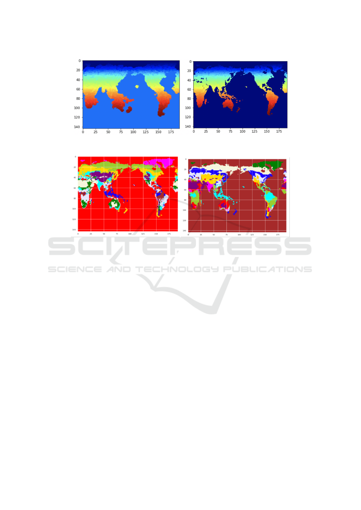
Figure 1: Left: Segments (colored according to latitude) after first application of Felzenszwalb’s algorithm. Right: Segments
after second pass, and removal of segments with no terrestrial biomes (see text).
Figure 2: Left: Clustering without using segmentation. Right: Clustering after using segmentation. The colors distinguish
clusters, and have no other significance.
approach is composed of the following steps:
1. Rescale the data and stack it into a tensor.
2. Use Felzenszwalb’s segmentation algorithm
(Felzenszwalb and Huttenlocher, 2004) on the
tensor data to decompose it into regions. This step
helps to produce smoother biomes and alleviates
the effects of outliers without removing them.
3. Transform the newly formed segments into a tab-
ular dataset D where each segment represents a
row of data. The values of each row are the me-
dian values of the pixels’ segments.
4. Use k-means to cluster D into k clusters.
5. Produce a decision tree taking the inputs as the
dataset D and the labels as the k cluster identifiers
(or pseudo-labels) with a set of hyper-parameters
allowing a good compromise between accuracy
and interpretability.
We give details about each step of our approach in the
following sections.
4.1 Data Pre-processing
Our dataset consists of 15 global land surface vari-
ables on a latitude-longitude N96 climate model grid
whose dimensions are 180 (longitude) by 142 (lati-
tude). We recale each variable and then stack them at
each grid cell to produce an image whose pixels have
15 channels. This can be viewed as a 3D tensor whose
dimensions are longitude, latitude and channel.
4.2 Processing Outliers
Some pixels may contain values that could be consid-
ered as outliers, or noise resulting from errors associ-
ated with the data or other conditions. If we cluster
such pixels into groups, neighbouring pixels will be-
long to different clusters which will result in a grained
distribution—for example, tiny clusters represented
by individual pixels within a large cluster. Figure 1
represents such phenomena. To alleviate the effects
of outliers, we use an image segmentation-based ap-
proach. Although our data are not images in the con-
ventional sense, they have an analogous structure—
i.e our data points have a two-dimensional spatial re-
lationship in which proximity and location is signifi-
cant.
Image segmentation methods decompose images
into regions whose pixels have similar characteristics.
The pixels within every segment are rather similar but
Explainable Clustering Applied to the Definition of Terrestrial Biomes
589

not identical. They also tend to be localized (i.e pixels
which are far apart are unlikely to be part of the same
segment).
We chose Felzenszwalb’s (Felzenszwalb and Hut-
tenlocher, 2004) algorithm as a segmentation that
does not require a fixed number of segments in ad-
vance (unlike SLIC superpixels (Achanta et al., 2012)
for example). Felzenszwalb is a graph-based algo-
rithm that ignores low variabilities in high variability
regions, resulting in segments which appear more nat-
ural. There is no restriction on the shape of the seg-
ments it produces. While images encoded as matrices
typically have three channels (e.g. RGB, or HSL val-
ues), there are no restrictions on the number of chan-
nels this algorithm can work with.
Applying Felzenszwalb’s algorithm with the pa-
rameters values scale = 0.4, sigma = 0.5, minsize = 3
produces 1663 segments (see left hand side of Fig-
ure 1). The scale parameter controls the size of
the segments—larger values produce larger segments.
minsize is the minimum number of pixels which each
segment can contain, and sigma is a pre-processing
parameter that controls the dimensions of the Gaus-
sian kernel. Close inspection reveals that certain
small non-terrestrial (water) regions were mistaken
for noise due to their small size. A second pass of the
segmentation method grouped these non-terrestrial
regions into one segment, which we then removed
(along with segments corresponding to Antarctica)
since these regions have no terrestrial biomes of in-
terest. The right hand side of Figure 1 shows the 1216
segments which remained after this removal; compar-
ing the two sides of the figure shows the improvement
in the resolution of the coastline arising from the re-
moval of the non-terrestrial regions.
15 values characterise each segment—that is, the
median of each of the 15 variables within the seg-
ment’s boundary.
v
k
(segment
i
) = median(x
ki j
) (1)
where v
k
is variable k’s value for segment
i
, j is a point
index within its segment, and x
ki j
is the value of vari-
able k of data point j belonging to segment i.
4.3 Clustering the Map via k-Means
K-means is a distance-based algorithm that groups
points with similar feature values by assigning each
point to the cluster with the nearest centroid. It finds
centroids that minimise the sum of the squared Eu-
clidean distance between each data point and its asso-
ciated centroid:
argmin
m
∑
i=0
||x
i
− µ
c
i
||
2
(2)
Figure 3: A plot of gap value against cluster count. This is
one of the methods used to determine a suitable cluster size
(see text).
where x
i
are the vectors representing data points i and
µ
c
i
are the centroid vectors associated with data point
i.
We used k-means with all 15 variables for our
analysis. We acknowledge that some of these vari-
ables are correlated as they are influenced by the same
underlying physical processes and that such correla-
tions might determine cluster associations. However,
we did not see any evidence that the semantic integrity
of our clusters was significantly impacted by these
correlations and so we chose to retain all 15 variables.
The k-means clustering algorithm requires the
number of clusters (that is, k) as one of the hyper-
parameters. The selection of a value for this param-
eter requires some consideration. For example, we
could set it to the number of biomes used in an em-
pirical characterization approach for comparative pur-
poses, or to a higher or lower value to obtain a more
generalized or more granular result. We employed
three different evaluation metrics to estimate the op-
timal number of clusters: the Distortion Coefficient,
Gap values and the Silhouette score. We show an
illustration of how we employed one of the metrics
(Gap values) in Figure 3. Based on this metric, we de-
termined that a number between 10 and 15 (clusters)
would optimally represent our data. We found that the
Distortion Coefficient and the Silhouette scores were
in agreement with this range, suggesting a compara-
ble number of clusters.
We finally chose to employ 11 clusters for defin-
ing biomes in this approach – a number consistent
with both expectations from domain-expertise and the
evaluation metrics we employed.
4.4 Tree-based Interpretability
Machine learning models that are not easy to ex-
plain in simple terms require the application of spe-
cific extra methods, including SHAP (SHapley Ad-
ICPRAM 2022 - 11th International Conference on Pattern Recognition Applications and Methods
590
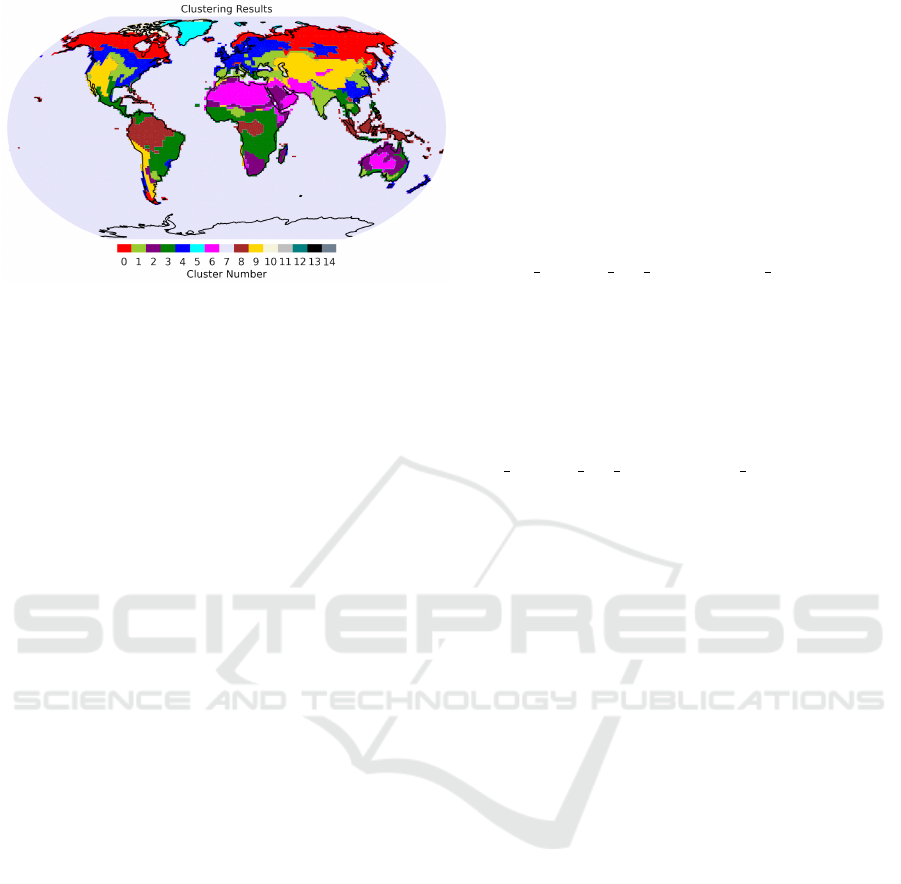
Figure 4: Results of k-means clustering algorithm, identi-
fying 11 biomes. The key distinguishes 14 clusters, but not
all of them are present.
ditive exPlanations) (Lundberg and Lee, 2017) and
LIME (Local Interpretable Model-agnostic Explana-
tions) (Ribeiro et al., 2016). Models which are more
explainable (for example, a decision tree with a com-
paratively low depth) do not need methods such as
these to be applied. Such models include decision
trees, linear regressions and na
¨
ıve Bayes. These mod-
els belong to the supervised learning family. Explain-
able models in clustering and unsupervised learning
in general are very scarce.
Decision rules provide an explainable way to de-
fine categories. Each category is bounded by a set
of conditions, generally Boolean. A number of al-
gorithms exist that can generate decision rules for a
given problem. (Chavent, 1998) builds decision rules
directly for clustering purposes on unlabelled data. It
uses a similarity measure to decide on dividing clus-
ters of data by finding the optimal splitting value on
features. The process is similar to the splits used in
decision trees. The method builds hyper-cubic shaped
clusters but does not put a restriction on the number
of rules or the number of features used. This method
optimises the decisions at each level instead of opti-
mising the whole structure of the clusters. (Dasgupta
et al., 2020) uses first k-means to build clusters, and
then builds a minimum set of decision rules on top
of these clusters to approximate them. The simpler
the rules, and the smaller the set, the more explain-
able the clustering will be. Another method of build-
ing explainable clustering is to approximate k-means
clusters with a decision tree while restricting the size
of the tree via its hyper-parameters. We use this ap-
proach. Since decision boundaries in decision trees
are made of vertical and horizontal lines and k-means
clusters boundaries are spherical-like, we would not
expect them to be exactly equivalent. Instead, we
choose hyper-parameters that allow a good compro-
mise between interpretability and equivalence. We
define two models as equivalent if they assign the
same label (or cluster) to a given data point—i.e. if
the models agree on the classification of all the data
points. We adopt the following algorithm to generate
interpretable decision trees:
1. Generate k clusters using k-means (see §4.3). Re-
sults are presented in figure 4.
2. Use the resultant clusters identifiers as pseudo la-
bels for the data.
3. Build a decision tree using:
min samples per node=30, max depth=9
4. Recursively trim the resulting tree if the predicted
classes do not change in sibling leaves
It is worth noting that there is a set of de-
cision trees that can approximate the clustering
results while producing explainable rules. The
above algorithm generates one among several pos-
sibilities. Tweaking the hyper-parameters such as
min samples per nodes and max depth will produce
slightly different trees. We note that the algorithms
we used to build the trees are (Breiman et al., 2017)
and C4.5 (Quinlan, 2014), other clustering or tree-
based algorithms will produce different trees.
(Dasgupta et al., 2020) describe a k-means cluster-
ing result along with a possible decision tree approxi-
mation. Our aim here, however is to explore the effect
of the addition of interpretability to k-means cluster-
ing, in particular whether it enhances the comparison
with results from empirical classification methods for
terrestrial biomes. To better satisfy interpretability,
we have two goals that will guide us during the tree’s
construction. The first one is to produce short rules,
which is equivalent to the decision tree length. The
second aim is to reduce the number of rules per clus-
ter to as close to one as possible. These goals will help
deliver the definition of biomes in a fashion which
is more accessible to the domain knowledge experts
who can examine, strip, augment, or even discard
them. Such rules will also be comparable in struc-
ture to the empirical rules from models such as KG
tree or expert knowledge such as (Olson et al., 2001).
4.5 Results
Having applied the methodology described in (§§4.1–
4.4) to generate explainable biomes, we present our
results and compare them to those from the empirical
biome attributions. Upon a partial application of our
method, without selecting the hyper-parameters that
account for short and small numbers of rules and tree
trimming, the resultant decision tree (called TreeA)
approximates k-means clustering with an agreement
of 95%. Although the decision tree gives a very good
Explainable Clustering Applied to the Definition of Terrestrial Biomes
591
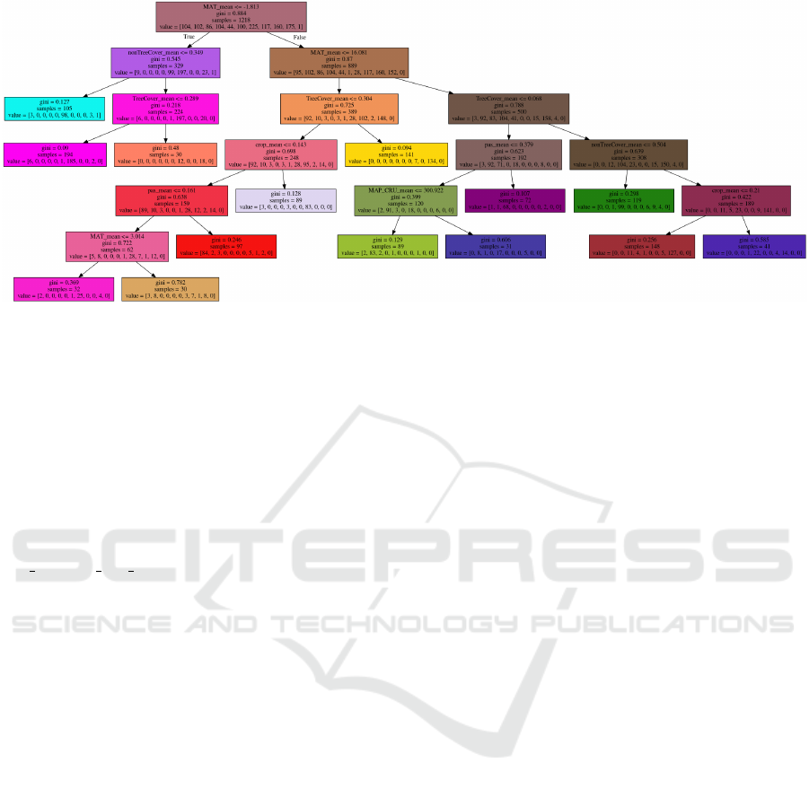
Figure 5: Final reduced decision tree after application of recursive trimming algorithm (i.e. TreeB), resulting in 14 leaf nodes.
representation of the original clusters, it uses around
80 rules to define all the biomes. This is a compara-
tively large number, representing a challenge for the
usability of the classification scheme, and for compar-
isons with the results from the empirical characteriza-
tion approach. Therefore, we compromise agreement
with the clusters and usability by setting values for
the hyper-parameters in the decision tree algorithm,
defining the minimum number of samples per leaf
min samples per nodes to 30, limiting the tree depth.
We also recursively trim the tree, using the following
algorithm:
Order pairs of sister leaves based on length
for each pair of sister leaves a,b:
if majority_class(a) == majority_class(b):
c=merge(a,b)
d=find_sister_leaf(c)
insert pair(c,d) in list of sister
leaves keeping the order
end
Applying the algorithm with the hyper-parameter
values mentioned above and using recursive trim-
ming produces decision tree TreeB which is in 85%
agreement with the original clusters. However, the
tree contains 14 leaves, which makes it considerably
smaller than TreeA—see Figure 5. In a trimmed tree
all biomes (except three) are explained by a single leaf
and thus a single rule. This supports the hypothesis
that most biome definitions can be defined in an ex-
plainable way. We then re-clustered the regions of the
map according to TreeB. In this tree, leaves are num-
bered from 0 to 10. Leaves are assigned to biomes
according to the index of the maximum value in the
leaf’s segments array—for example, a leaf with seg-
ments array of [2, 55, 3, 0, 1, 0, 4, 4, 1, 1, 0] would rep-
resent biome 1.
5 DISCUSSION
By comparing our results to the empirical biomes de-
fined by experts in the literature, we can observe a
number of biomes that are in accordance with our re-
sults such as the tropical rainforest, the tundra, the
taiga, the desert, the steppe, the savanna and the
mixed forest with some variations on their bound-
aries. However, we also observe a couple of extra
biomes, one of which is mainly present in the Indian
subcontinent, while the other is a semi-arid biome
similar to desert. The biome present in the Indian sub-
continent seems to be influenced by agriculture and
suggests an anthropogenically-induced change. Fur-
ther analysis of these results is required to compare
the boundaries of the discovered biomes to those de-
rived by empirical methods. Figure 7 shows a com-
parison between Olson’s biomes (Olson et al., 2001)
and the biomes derived from the explainable cluster-
ing methodology. Typically there is a strong overlap
between our derived biomes and those from Olson
(for example, the desert biome has a 92% overlap,
tropical forest has 87%). Interestingly, when there is
some disagreement, a biome is still often attributed
as belonging to a similar biome (e.g. boreal forest
and tundra) suggesting the boundary between biomes
is somewhat fluid. Applying an image segmenta-
tion algorithm helped in making biomes more con-
tinuous in space, thus ignoring localized small vari-
ations. An examination of the decision rules and t-
distributed stochastic neighbour embedding (t-SNE)
visualizations of the biomes reveals the following:
• Most biomes require only one rule to define them.
• Two leaves do not have a clear majority decision.
• Three biomes (biomes number 4, 6 and 9) each
ICPRAM 2022 - 11th International Conference on Pattern Recognition Applications and Methods
592
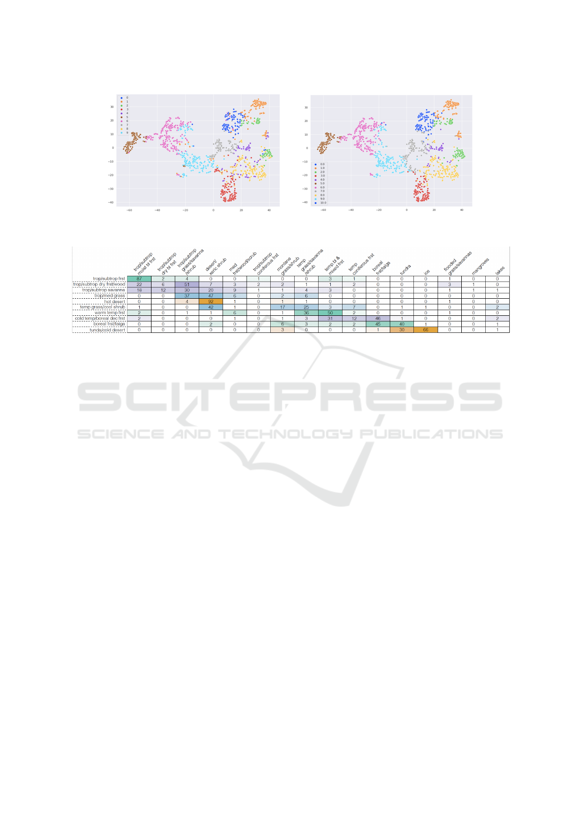
(a) t-SNE projection for the final clusters (b) t-SNE projection for k-means clusters
Figure 6: t-SNE projections.
Figure 7: A comparison of biomes obtained from explainable clusters against Olson’s biomes (Olson et al., 2001). The
numbers show the % of clustering biomes that fall in each Olson biome. In biome names, trop = tropical, med = Mediterranean,
frst = forest, wood = woodland, shrub = shrubland, shrub = scrubland, grass = grassland, bl = broadleaf. The color of each cell
denotes the type of biome (green = forest, blue = woodland, purple = grassy, orange = barren); color intensity is proportional
to the value in the cell.
require two rules to be defined.
Biome 6 (represented by the pink leaves in Figure
5) covers a large part of the map. Most of its region
is governed by a single rule covering 185 segments
from the map, whilst the second rule covers only 25
segments. The 25 segments appear to be close to the
borders with other biomes.
Similarly, biome 9 represented by the yellow leaf
is defined by two rules as well. One rule governs 134
segments, while the other governs 18 segments and
another 12 segments from biome 6. Both rules are
characterized by a high tree coverage and adjacent in-
tervals of mean annual temperatures. This may allow
these two rules to be fused in one single rule.
Looking at the t-SNE plot in figure 6 of the de-
cision tree, we note that biomes 1 and 4 are highly
mixed with other biomes in the spatial representation
while the t-SNE graph of the k-means clusters does
not shows this mixtures. This suggests that these two
biomes may not be easily defined by simple rules.
Biome 1 which appears to represent the desert is less
prone to this effect than biome 4. The latter, which
to date appears to be the only biome that the decision
tree approach is unable to identify. The fact that it
is related to agricultural regions suggests that “non-
natural” biomes may not follow the same structure as
the others, and the effect of these man-made environ-
mental changes are more complex than those repre-
sented by natural observable features. Biome 4 ap-
pears to share some characteristics with neighbour-
ing biomes but is sufficiently different to be charac-
terized as a new biome by k-means. However, it is
not distinctive enough to be fully explainable. We
note that most of the other irregularities in the deci-
sion tree-based clustering are located near the borders
of biomes in data space.
We also note that decision trees that can approx-
imate k-means are not unique. For this, a further
analysis of the different ways of approximating the
k-means clusters is required. For example, changing
the weights of certain instances will result in a differ-
ent tree with a possibility of a different interpretability
level. There are also tree construction methods that
are not based on CART or C4.5 such as the methods
presented in (Dasgupta et al., 2020) that can applied
to this use case.
6 CONCLUSION
In this work we have defined a methodology for ex-
plainable clustering which we have applied to 3D ten-
sor data. Our motivation is the production of explain-
able definitions of terrestrial biomes. After rescaling
Explainable Clustering Applied to the Definition of Terrestrial Biomes
593

the data, we superpose them as 3D tensors and ap-
ply an image segmentation algorithm to decompose
the tensor into homogeneous segments. We apply k-
means clustering to the segments, and introduce ex-
plainability by approximating the clusters with a de-
cision tree, which we subsequently trim to a manage-
able number of leaves.
This method allowed for the building of continu-
ous biomes in space with one rule per biome in most
cases. Three biomes required more than one rule to
define them. Four of these rules could be fused into
two rules thus making the clustering simpler. How-
ever, despite using all 15 features in the construction
of the decision tree, the resulting rules used at most
four features. This is due to underlying latent fea-
tures influencing more than one correlated feature.
It is worth noting that a decision tree which is rel-
atively small and can approximate clustered data is
not unique. Different methods with different hyper-
parameters will produce different trees. We also no-
ticed that certain biomes that are man-made such as
the Indian subcontinent biome cannot be easily de-
fined by rules without affecting the rules of adjacent
biomes. This indicates that this biome has an irregular
shape (in data space) and indeed requires more than
one rule to be defined. One final observation is that
decision trees are not perfect in building simple rules
for clustering. Because rules are constrained to be
connected at different node levels, simplicity may be
traded for this property. For future work, we suggest
augmenting this method with a strategy for merging
rules that not only merges rules when they are con-
nected via a feature but also when features are corre-
lated and there is a possibility for such a merge. These
may lead to a loss in precision depending on the cor-
relation level but it will improve the interpretability.
We believe that this study demonstrates the strong
potential possible for advancing our understanding of
Earth system science by utilising machine learning
methods, such as explainable clustering. By expand-
ing this work in the future and applying these methods
to climate projections from Earth system models, we
will be able to provide analyses which complement
existing insights from experts about how the Earth’s
biomes may alter in response to a changing climate.
7 DATA AVAILABILITY
The data used (Table 1) are archived at
https://doi.org/10.5281/zenodo.5736407 (Kelley
et al., 2021b).
ACKNOWLEDGEMENTS
This project originated as a collaboration between the
Met Office and Amazon Web Services (AWS) under
the AWS Machine Learning Embark program. JW
is supported by the Met Office Hadley Centre Cli-
mate Programme funded by BEIS and Defra. RS
and RJP are funded by the UK National Centre for
Earth Observation (UKESM, NE/N018079/1). DIK
was supported by the UK Natural Environment Re-
search Council (UKESM, NE/N017951/1).
REFERENCES
Achanta, R., Shaji, A., Smith, K., Lucchi, A., Fua, P., and
S
¨
usstrunk, S. (2012). SLIC superpixels compared to
state-of-the-art superpixel methods. IEEE Transac-
tions on Pattern Analysis and Machine Intelligence,
34(11):2274–2281.
Adzhar, R., Kelley, D. I., Dong, N., Torello Raventos, M.,
Veenendaal, E., Feldpausch, T. R., Philips, O. L.,
Lewis, S., Sonk
´
e, B., Taedoumg, H., Schwantes Ma-
rimon, B., Domingues, T., Arroyo, L., Djagbletey, G.,
Saiz, G., and Gerard, F. (2021). Assessing MODIS
Vegetation Continuous Fields tree cover product (col-
lection 6): performance and applicability in tropical
forests and savannas. Biogeosciences Discussions,
2021:1–20.
Ben-Dor, A., Shamir, R., and Yakhini, Z. (1999). Clustering
gene expression patterns. Journal of computational
biology, 6(3-4):281–297.
Breiman, L., Friedman, J. H., Olshen, R. A., and Stone,
C. J. (2017). Classification and regression trees. Rout-
ledge.
Chavent, M. (1998). A monothetic clustering method. Pat-
tern Recognition Letters, 19(11):989–996.
Dasgupta, S., Frost, N., Moshkovitz, M., and Rashtchian,
C. (2020). Explainable k-Means Clustering: Theory
and Practice. In XXAI Workshop, ICML.
Davis, T. W., Prentice, I. C., Stocker, B. D., Thomas,
R. T., Whitley, R. J., Wang, H., Evans, B. J., Gallego-
Sala, A. V., Sykes, M. T., and Cramer, W. (2017).
Simple process-led algorithms for simulating habitats
(SPLASH v.1.0): Robust indices of radiation, evapo-
transpiration and plant-available moisture. Geoscien-
tific Model Development, 10(2):689–708.
DeSantis, D., Wolfram, P. J., Bennett, K., and Alexan-
drov, B. (2020). Coarse-grain cluster analysis of
tensors with application to climate biome identifica-
tion. Machine Learning: Science and Technology,
1(4):045020.
Dimiceli, C., Carroll, M., Sohlberg, R., Kim, D. H., Kelly,
M., and Townshend, J. R. G. (2015). MOD44B
MODIS/Terra Vegetation Continuous Fields Yearly
L3 Global 250m SIN Grid V006 (V006).
Felzenszwalb, P. F. and Huttenlocher, D. P. (2004). Effi-
ICPRAM 2022 - 11th International Conference on Pattern Recognition Applications and Methods
594

cient graph-based image segmentation. International
Journal of Computer Vision, 59(2):167–181.
Forrest, M., Tost, H., Lelieveld, J., and Hickler, T. (2020).
Including vegetation dynamics in an atmospheric
chemistry-enabled general circulation model: Link-
ing LPJ-GUESS (v4.0) with the EMAC modelling
system (v2.53). Geoscientific Model Development,
13(3):1285–1309.
Harris, I. (2019). CRU JRA v1. 1: A forcings dataset of
gridded land surface blend of Climatic Research Unit
(CRU) and Japanese reanalysis (JRA) data, January
1901–December 2017, University of East Anglia Cli-
matic Research Unit, Centre for Environmental Data
Analysis.
Harris, I. and Jones, P. (2017). CRU TS4. 01: Climatic Re-
search Unit (CRU) Time-Series (TS) version 4.01 of
high-resolution gridded data of month-by-month vari-
ation in climate (Jan. 1901–Dec. 2016). Centre for
Environmental Data Analysis, 25.
Hartigan, J. A. and Wong, M. A. (1979). Algorithm AS 136:
A K-Means Clustering Algorithm. Applied Statistics,
28(1):100.
Johnson, S. C. (1967). Hierarchical clustering schemes.
Psychometrika, 32(3):241–254.
Kaufman, L. and Rousseeuw, P. (1987). Clustering by
means of Medoids. In Statistical Data Analysis Based
on the L1 Norm and Related Methods, pages 405–416,
North-Holland. Y. Dodge, Ed.
Kelley, D., Gerard, F., Dong, F., Whitley, R., Li, G., Burton,
C., Marthews, M., Weedon, G., Lasslop, G., Ellis, R.,
Bistnas, I., and Veendendaal, E. (2021a). Revisiting a
”World Without Fire”: Low influence of fire on tropi-
cal tree cover. Submitted.
Kelley, D. I., Bistinas, I., Whitley, R., Burton, C., Marthews,
T. R., and Dong, N. (2019). How contemporary biocli-
matic and human controls change global fire regimes.
Kelley, D. I., Dong, N., Li, G., Sidoumou, M. R., Kim,
A., Walton, J., Parker, R. J., and Swaminathan, R.
(2021b). Explainable Clustering Applied to the Defi-
nition of Terrestrial Biomes - data.
Klein Goldewijk, K., Beusen, A., Van Drecht, G., and De
Vos, M. (2011). The HYDE 3.1 spatially explicit
database of human-induced global land-use change
over the past 12,000 years. Global Ecology and Bio-
geography, 20(1):73–86.
Kottek, M., Grieser, J., Beck, C., Rudolf, B., and Rubel,
F. (2006). World Map of the K
¨
oppen-Geiger climate
classification updated. Meteorologische Zeitschrift,
15(3):259–263.
Lloyd, S. (1982). Least squares quantization in PCM. IEEE
transactions on information theory, 28(2):129–137.
Lundberg, S. M. and Lee, S. I. (2017). A unified approach
to interpreting model predictions. In Advances in Neu-
ral Information Processing Systems, volume 2017-
Decem, pages 4766–4775.
Mahalanobis, P. C. (1936). On the generalised distance in
statistics. Proceedings of the National Institute of Sci-
ences of India, 2(1):49–55.
Netzel, P. and Stepinski, T. (2016). On using a clustering
approach for global climate classification. Journal of
Climate, 29(9):3387–3401.
Olson, D. M., Dinerstein, E., Wikramanayake, E. D.,
Burgess, N. D., Powell, G. V. N., Underwood, E. C.,
D’amico, J. A., Itoua, I., Strand, H. E., Morrison,
J. C., Loucks, C. J., Allnutt, T. F., Ricketts, T. H.,
Kura, Y., Lamoreux, J. F., Wettengel, W. W., Hedao,
P., and Kassem, K. R. (2001). Terrestrial Ecoregions
of the World: A New Map of Life on Earth: A new
global map of terrestrial ecoregions provides an inno-
vative tool for conserving biodiversity. BioScience,
51(11):933–938.
Peel, M. C., Finlayson, B. L., and McMahon, T. A. (2007).
Updated world map of the K
¨
oppen-Geiger climate
classification. Hydrology and Earth System Sciences,
11(5):1633–1644.
Prentice, I. C., Harrison, S. P., and Bartlein, P. J. (2011).
Global vegetation and terrestrial carbon cycle changes
after the last ice age. New Phytologist, 189(4):988–
998.
Quinlan, J. R. (2014). C4.5: Programs for Machine Learn-
ing. Elsevier.
Ribeiro, M. T., Singh, S., and Guestrin, C. (2016). ”Why
should I trust you?” Explaining the predictions of any
classifier. In Proceedings of the ACM SIGKDD In-
ternational Conference on Knowledge Discovery and
Data Mining, volume 13-17-Augu, pages 1135–1144.
Association for Computing Machinery.
Sato, H., Kelley, D. I., Mayor, S. J., Martin Calvo, M.,
Cowling, S. A., and Prentice, I. C. (2021). Dry corri-
dors opened by fire and low CO2 in Amazonian rain-
forest during the Last Glacial Maximum. Nature Geo-
science, 14:578–585.
Sellar, A. A., Jones, C. G., Mulcahy, J. P., Tang, Y., Yool,
A., Wiltshire, A., O’Connor, F. M., Stringer, M.,
Hill, R., Palmieri, J., Woodward, S., de Mora, L.,
Kuhlbrodt, T., Rumbold, S. T., Kelley, D. I., Ellis, R.,
Johnson, C. E., Walton, J., Abraham, N. L., Andrews,
M. B., Andrews, T., Archibald, A. T., Berthou, S.,
Burke, E., Blockley, E., Carslaw, K., Dalvi, M., Ed-
wards, J., Folberth, G. A., Gedney, N., Griffiths, P. T.,
Harper, A. B., Hendry, M. A., Hewitt, A. J., John-
son, B., Jones, A., Jones, C. D., Keeble, J., Liddicoat,
S., Morgenstern, O., Parker, R. J., Predoi, V., Robert-
son, E., Siahaan, A., Smith, R. S., Swaminathan,
R., Woodhouse, M. T., Zeng, G., and Zerroukat, M.
(2019). UKESM1: Description and Evaluation of the
U.K. Earth System Model. Journal of Advances in
Modeling Earth Systems, 11(12):4513–4558.
Thornthwaite, C. W. (1948). An Approach toward a Ratio-
nal Classification of Climate. Geographical Review,
38(1):55.
Van Der Werf, G. R., Randerson, J. T., Giglio, L.,
Van Leeuwen, T. T., Chen, Y., Rogers, B. M., Mu, M.,
Van Marle, M. J., Morton, D. C., Collatz, G. J., et al.
(2017). Global fire emissions estimates during 1997–
2016. Earth System Science Data, 9(2):697–720.
Ward, J. H. (1963). Hierarchical Grouping to Optimize an
Objective Function. Journal of the American Statisti-
cal Association, 58(301):236–244.
Explainable Clustering Applied to the Definition of Terrestrial Biomes
595
