Highways in Warehouse Multi-Agent Path Finding: A Case Study

Vojt

ech Ryb

and Pavel Surynek

Faculty of Information Technology, Czech Technical University, Th

akurova 9, 160 00 Praha 6,Czech Republic

Keywords:

Multi-Agent Path Finding (MAPF), Highways, Conﬂict-Based Search (CBS).

Abstract:

Orchestrating warehouse sorting robots each transporting a single package from the conveyor belt to its des-

tination is a NP-hard problem, often modeled Multi-agent path-ﬁnding (MAPF) where the environment is

represented as a graph and robots as agents in vertices of the graph. However, in order to maintain the speed

of operations in such a setup, sorting robots must be given a route to follow almost at the moment they obtain

the package, so there is no time to perform difﬁcult ofﬂine planning. Hence in this work, we are inspired by

the approach of enriching conﬂict-based search (CBS) optimal MAPF algorithm by so-called highways that

increase the speed of planning towards on-line operations. We investigate whether adding highways to the

underlying graph will be enough to enforce global behaviour of a large number of robots that are controlled

locally. If we succeed, the slow global planning step could be omitted without signiﬁcant loss of performance.

1 INTRODUCTION

Logistics centres that are organised in such a way that

small sorting robots can operate in them, are starting

to become widespread. Their undeniable advantages

include higher speed in sorting larger quantities of

shipments and signiﬁcant savings in human labour.

Such logistics centres are organized the following

way: a human operator or a robot arm takes a package

from, e.g., a conveyor belt. Then the operator (robot

arm) uses the optical recognizing system to examine

the package to determine its destination cage. Then

the operator (robot arm) loads the package to a sorting

robot which is capable of carrying just one package.

Once the sorting robot is loaded with the package, it

takes off for its destination. When the sorting robot

arrives at its destination, it unloads the carried pack-

age to a hole in the ground, which is an entrance to a

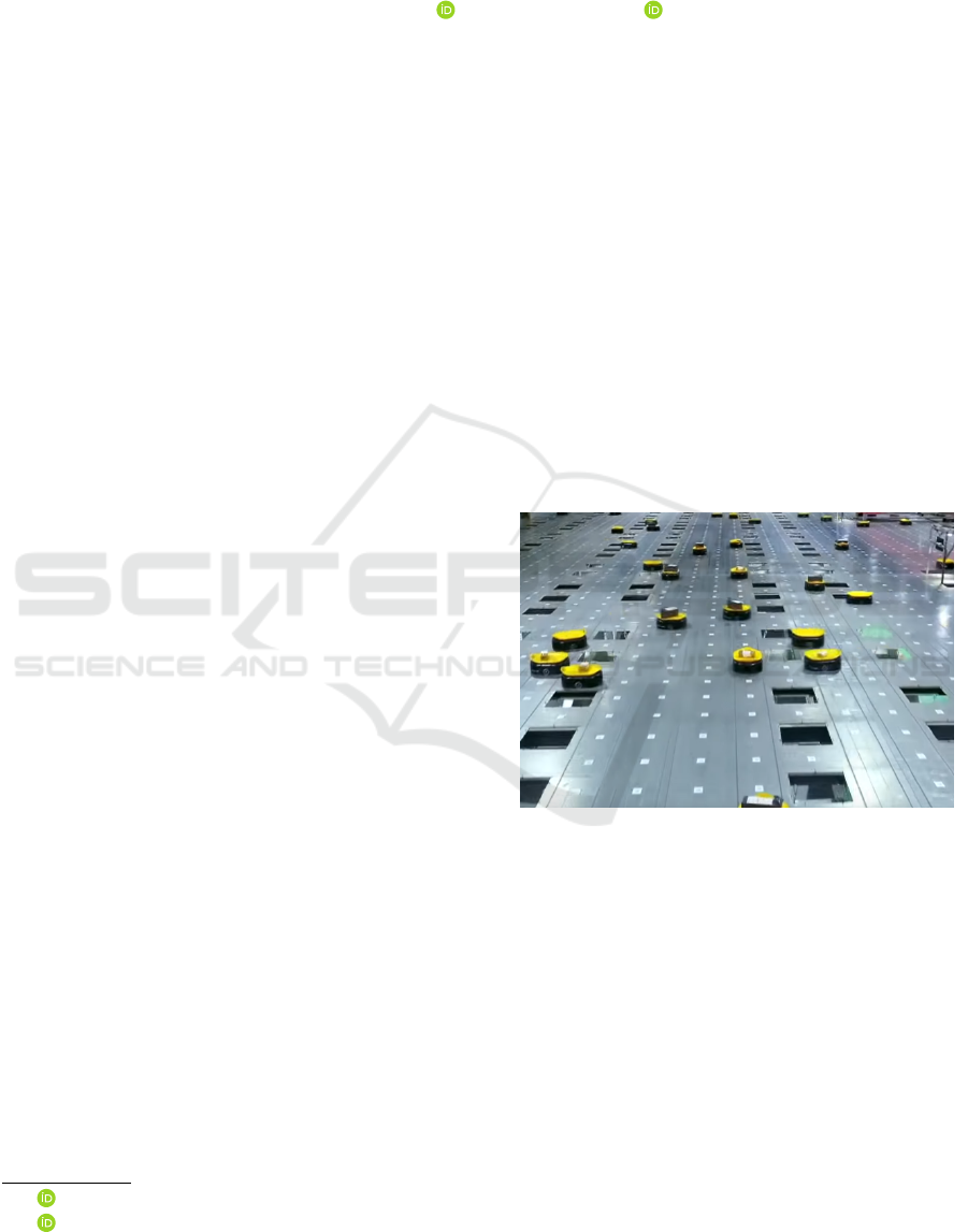
cage below the ﬂoor. We present a screenshot taken

from an illustrative YouTube video

in Figure 1.

This approach, where the operator stands in one

place and the robots with the load come to him and

leave again after the operator performs a simple op-

eration, was popularized by the Kiva robots (Wurman

et al., 2008). In contrast to them, the sorting robot we

consider in this paper only transports a single package

at a time.

https://orcid.org/0000-0003-0552-3997

https://orcid.org/0000-0001-7200-0542

https://youtu.be/jwu9SX3YPSk

Figure 1: Real world instance of the warehouse sorting

robots concept.

To ensure that the process of planning the individ-

ual routes of each sorting robot does not cause delays

that slow down the orchestration of the entire sort-

ing process in the logistics centre (and thus largely

reduce the main advantage of why logistics centres of

this type are being built), it is necessary that ﬁnding

the route for each robot, whether from where it has

been assigned a parcel and a destination cage, or back

to where it can load a new parcel, is a matter of mo-

ments.

As it makes no sense to employ just one sorting

robot in the whole warehouse, it is important to ﬁnd

a suitable route that would take into account other

robot operations in the same warehouse space. This

routing problem in the warehouse can be abstracted

274

Rybá

r, V. and Surynek, P.

Highways in Warehouse Multi-Agent Path Finding: A Case Study.

DOI: 10.5220/0010845200003116

In Proceedings of the 14th International Conference on Agents and Artiﬁcial Intelligence (ICAART 2022) - Volume 1, pages 274-281

ISBN: 978-989-758-547-0; ISSN: 2184-433X

as so-called Multi-agent path ﬁnding (MAPF) (Ryan,

2007; Silver, 2005; Kornhauser et al., 2009; Surynek,

2009). The task in MAPF is to navigate agents in a

graph from their starting vertices to given individual

goal vertices so that agent do not collide with each

other (that is, they neither share a vertex nor traverse

an edge in the opposite directions).

Such a problem has an optimal solution in terms

of the number of actions (movements), but ﬁnding

the optimal solution is NP-hard (Yu and LaValle,

2013; Surynek, 2010). With dozens to hundreds sort-

ing robot operation in current warehouses, this is a

substantial limitation. Conﬂict-Based Search (CBS)

(Sharon et al., 2015a) or SAT (Surynek, 2019) can

serve as well-established algorithms to obtain a glob-

ally optimal solution.

In this paper, we would like to compare how an

optimal solution obtained by the CBS algorithm per-

forms compared to the most simple algorithm we

could deﬁne that would ensure that robots do not

block each other so that their planned routes and col-

lision avoidance make movement around the ware-

house impossible.

Our approach is inspired by (Cohen and Koenig,

2016). There the authors enhance low-level CBS

search (explained in Section 2.1) with predeﬁned

preferable set of edges called highways. The second

source of inspiration is agent-based modeling (ABM)

(Castiglione, 2009) which aims at achieving complex

global behaviour of a group of agents via local con-

trol of individual agents. Here the behaviour we want

to achieve is that agents reduce collisions with each

other and the cost of the global plan is close to the

optimum.

We use the highway idea but remove the the global

planning step. All edges in our warehouse abstraction

(described in Section 3) will be made directed. In-

stead of global planning, each robot will check the

robots in its neighbourhood to avoid collisions. Thus

will follow simple local rules, however the environ-

ment is enhanced via highways which we believe can

make these simple rules efﬁcient.

1.1 Related Work

There are many approaches to solving optimalthe

MAPF problem optimally as well as bounded sub-

optimally. The solutions may be found via reduction

(often also called compilation) of the MAPF problem

to propositional satisﬁability (SAT) (Kautz and Sel-

man, 1999; Surynek et al., 2016) or to other estab-

lished formalism for modeling and solving NP-hard

problems (Lam et al., 2019)

Different stream of approaches is represented by

search-based algorithms that model the MAPF di-

rectly and suggest dedicated algorithm. Some of the

state-of-the-art algorithms include Increasing Cost

Tree Search - ICTS (Sharon et al., 2013), Conﬂict-

based Search - CBS (Sharon et al., 2015b), and Im-

proved CBS – ICBS (Boyarski et al., 2015) and mode.

Most of optimal algorithms have their bounded sub-

optimal variants that trade-off optimality for the speed

of solving.

2 MULTI-AGENT PATH FINDING

In MAPF, the time is discretized into time steps. The

conﬁguration of agents A = {a

,...,a

} in vertices

of the graph G = (V, E) at timestep t is denoted as s

Each agent a

has a start position s

) ∈ V and a goal

position s

) ∈ V .

Formally, a MAPF instance is a tuple Σ = (G =

(V,E),A,s

) where s

: R → V is an initial conﬁg-

uration of agents and s

: A → V is a goal conﬁgura-

tion of agents. A solution for Σ is a sequence of con-

ﬁgurations S (Σ) = [s

,...,s

] such that s

t+1

results

from valid movements from s

for t = 1,2,...,µ − 1,

and s

= s

. Orthogonally to this, the solution can be

represented as a set of paths for individual agents that

do not conﬂict with each other.

At each time step a agent can either move to an

adjacent location (vertex) or wait in its current loca-

tion. The task is to ﬁnd a sequence of move/wait ac-

tions for each agent a

, moving it from s

) to s

)

such that agents do not conﬂict, i.e., do not occupy

the same location at the same time and do not traverse

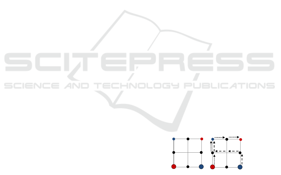
the same edge in opposite directions. An example of

MAPF instance and its solution is shown in Figure 2.

path(a

) =

, v

]

Cost = 4

path(a

) =

, v

]

Cost = 4

SoC = 8

MAPF

) = v

Figure 2: An MAPF instance with two agents a

and a

Often various cumulative objectives are optimized

in MAPF. We will develop all concepts in this paper

for the sum-of-costs objective, one of the most fre-

quently used, formally deﬁned as follows:

Deﬁnition 1. (Sum-of-Costs). Sum-of-costs denoted

SoC is the summation, over all agents, of the number

of time steps required to reach the goal. Formally,

SoC =

∑

i=1

cost(path(a

)), where cost(path(a

)) is

an individual path cost of agent a

connecting s

)

Highways in Warehouse Multi-Agent Path Finding: A Case Study

275

calculated as the number of edge traversals and wait

actions.

Observe that in the sum-of-costs we accumulate

the cost of wait actions for agents not yet reaching

their goal vertices. A feasible solution of a solvable

MAPF instance can be found in polynomial time (Ko-

rnhauser et al., 1984).

Finding an optimal solution with respect to the

sum-of-costs objective is NP-hard (Yu and LaValle,

2013; Surynek, 2010) and also determining the exis-

tence of a solution that differs from the optimum by a

factor less than 4/3 is NP-hard too (Ma et al., 2016).

Therefore designing algorithms based on search and

SAT for MAPF is justiﬁable.

2.1 Conﬂict-based Search

CBS is a representative of search-based approach.

CBS uses the idea of resolving conﬂicts lazily; that is,

a solution of MAPF instance is not searched against

the complete set of movement constraints that for-

bids collisions between agents but with respect to ini-

tially empty set of collision forbidding constraints that

gradually grows as new conﬂicts appear. The advan-

tage of CBS is that it can ﬁnd a valid solution before

all constraints are added.

The high level of CBS searches a constraint tree

(CT) using a priority queue in breadth ﬁrst manner.

CT is a binary tree where each node N contains a set

of collision avoidance constraints N.constraints - a

set of triples (a

,v,t) forbidding occurrence of agent

in vertex v at time step t, a solution N.paths - a set

of k paths for individual agents, and the total cost N.ξ

of the current solution.

The low level process in CBS associated with

node N searches paths for individual agents with re-

spect to set of constraints N.constraints. For a given

agent a

, this is a standard single source shortest path

search from α

) to α

) that avoids a set of

vertices {v ∈ V |(a

,v,t) ∈ N.constraints} whenever

working at time step t. For details see (Sharon et al.,

2015a).

CBS stores nodes of CT into priority queue OPEN

sorted according to ascending costs of solutions. At

each step CBS takes node N with the lowest cost from

OPEN and checks if N.paths represent paths that are

valid with respect to MAPF movements rules - that

is, N.paths are checked for collisions. If there is no

collision, the algorithms returns valid MAPF solution

N.paths. Otherwise the search branches by creating

a new pair of nodes in CT - successors of N. Assume

The notation path(a

) refers to path in the form of a

sequence of vertices and edges connecting s

) and s

)

while cost assigns the cost to a given path.

Algorithm 1: Basic variant of CBS algorithm for

MAPF solving.

1 CBS (G = (V,E),A,s

)

2 N.constraints ←

3 N.paths ← {shortest path from s

) to

)|i = 1, 2,...,k}

4 N.ξ ←

∑

i=1

ξ(N.paths(a

))

5 insert R into OPEN

6 while OPEN 6=

0 do

7 N ← min(OPEN)

8 remove-Min(OPEN)

9 collisions ← validate(N.paths)

10 if collisions =

0 then

11 return N.paths

12 let (a

,v,t) ∈ collisions

13 for each r ∈ {a

} do

14 N

.constraints ←

N.constraints ∪ {(r,v,t)}

15 N

.paths ← N.paths

16 update(r, N

.paths, N

.constraints)

17 N

.ξ ←

∑

i=1

ξ(N

.paths(a

))

18 insert N

into OPEN

that a collision occurred between agents a

and a

in vertex v at time step t. This collision can be

avoided if either agent a

or agent a

does not re-

side in v at timestep t. These two options cor-

respond to new successor nodes of N - N

and

that inherit set of conﬂicts from N as fol-

lows: N

.con f licts = N.con f licts ∪ {(a

,v,t)} and

.con f licts = N.con f licts ∪ {(a

,v,t)}. N

.paths

and N

.paths inherit paths from N.paths except those

for agents a

and a

respectively. Paths for a

and a

are recalculated with respect to extended sets of con-

ﬂicts N

.con f licts and N

.con f licts respectively and

new costs for both agents N

.ξ and N

.ξ are deter-

mined. After this, N

and N

are inserted into the pri-

ority queue OPEN.

The pseudo-code of CBS is listed as Algorithm 1.

One of crucial steps occurs at line 16 where a new

path for colliding agents a

and a

is constructed with

respect to the extended set of conﬂicts. N.paths(r)

refers to path of agent r.

The CBS algorithm ensures ﬁnding sum-of-costs

optimal solution. Detailed proofs of this claim can be

found in (Sharon et al., 2015a).

2.2 Highways

The planning part of Highway algorithm (HW) is de-

scribed in Algorithm 2. Lines 3-24 are plain A

∗

al-

gorithm. All notation is the same as in the CBS case

except the input H which is the heuristic to be used

for the in the A

∗

algorithm.

ICAART 2022 - 14th International Conference on Agents and Artiﬁcial Intelligence

276

Algorithm 2: Highway algorithm.

1 HW (G = (V,E),H, A,s

)

2 for each a

|i = 1, 2,...,k do

3 OPEN ← s

)

4 for each v ∈ V do

5 v

CAMEFROM

← NAN

6 v

← ∞

7 v

← ∞

8 s

)

← 0

9 while OPEN 6=

0 do

10 v ← o ∈ OPEN with smallest o

11 if v = s

) then

12 path ←

path from s

) to s

)

13 traversing CAMEFROM

14 return path

15 remove v from OPEN

16 for each n: {v,n} ∈ E do

17 g

tentative

← v

+ 1

18 if g

tentative

< n

then

19 n

CAMEFROM

← v

20 n

← g

tentative

21 n

← n

+ H(n)

22 if n /∈ OPEN then

23 OPEN ← OPEN ∪ {n}

24 return failure

Unlike the CBS algorithm, the Highway algo-

rithm does not produce conﬂict-free plans. Therefore,

conﬂicts need to be resolved during the simulation

run. Details of our implementation of avoiding col-

lisions are described in the following section where

the whole experimental body of work is introduced

and described.

For the Highway algorithm to work, we need the

graph edges of the graph G = (V, E) to be oriented.

Otherwise, robots with conﬂicting plans can easily

block each other from executing the next step. This

might happen as well in the case of the Highway al-

gorithm in a pathological conﬁguration of a graph and

number of agents. We observed this behaviour in the

second experiment described below. To avoid robots

blocking each other, we removed a couple of edges

from the underlying graph, the details are described

in the following sections and depicted in Figures 5

and 6.

In the Highway algorithm, we use as heuristics H

a zero vertex function H

deﬁned the following way:

(v) = 0 ∀v ∈ V.

Let us think for now of Algorithm 2 as an actual

implementation of line 3 in Algorithm 1.

Furthermore, let us construct an oriented subgraph

= (V

) of the graph G = (V,E) and de-

ﬁne the heuristics H

the following way:

(v) = min

∑

i+1

)∈π

(

1 if (s

i+1

) ∈ E

w otherwise,

where π = {v,...,s

)} ∈ V is a path from vertex v

to a robot destination s

) and w is a given constant.

If we use H

as the the heuristics in Algorithm 2

for implementation of line 3 in Algorithm 1, we will

get the original algorithm from (Cohen and Koenig,

2016).

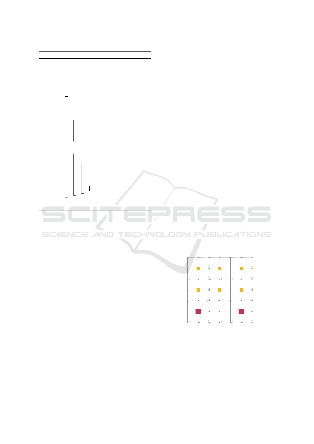
3 WAREHOUSE ABSTRACTION

For an abstraction of a physical world warehouse, we

use a rectangular planar graph as depicted in Figure

3. The graph can be either directed or undirected.

Whether we use directed or undirected edges depends

on the planning algorithm as described in the follow-

ing sections. Purple squares represent places where

an warehouse operator picks a single package from

a conveyor belt. Optical character recognition sys-

tem detects the nature and/or destination of the pack-

age, and then the sorting cage of the package is deter-

mined. When the unloaded agent arrives at the graph

node to the left of the loading spot, the operator loads

the package onto the sorting agent and the warehouse

system assigns the agent the proper destination cage.

Destination cages are depicted as yellow squares in

Figure 3. When the agent arrives at a graph node

above the destination cage, it unloads the package.

Then the agent destination is set to a loading spot.

Figure 3: Example of a planar graph used as an abstraction

of real-world warehouse where sorting agents can operate.

At each time step at every graph vertex, there can

be at most one agent. Moreover, one graph edge can

be used by only one agent at each time step, i.e.,

agents cannot swap locations in one step. Which

would make sense only in the case of undirected

graphs anyway.

Highways in Warehouse Multi-Agent Path Finding: A Case Study

277

Our model neglects several aspects of the real-

world scenario. We do not take into account any time

needed to load and unload the agent. In addition, ev-

ery agent move from one node of the graph to another

takes one time step. We are not taking into account ac-

celeration, deceleration, or direction change. Agents

need recharging from time, to time which is also not

in our consideration.

4 EXPERIMENTAL

COMPARISON

4.1 Agents.jl Implementation

We evaluated performance of the above-described

planning algorithms within the Agent-based mod-

elling paradigm where autonomous agents behave ac-

cording to a set of predeﬁned rules inside a computa-

tional simulation environment.

We implemented the abstraction from Section 3 in

Agents.jl (Datseris et al., 2021). Agents.jl is a frame-

work for agent-based modelling written in Julia with

three basic building blocks:

1. model deﬁnition,

2. model step function,

3. agent step function.

Julia programming language was chosen because

it is a ﬂexible programming language with perfor-

mance comparable to traditional statically-typed lan-

guages

Our warehouse abstraction can be deﬁned in

Agents.jl as a straightforward application of the pre-

deﬁned graph model block.

When CBS algorithm is employed, the model step

function ﬁnds a new plan every time a new destination

for any agent is determined. With HW, it does not

need to do anything.

In the case of CBS algorithm, the agent step func-

tion only makes the agent follow the central plan, i.e.,

move agent to the next vertex along the planned route.

In the case of HW, it ﬁnds the shortest path between

the starting point and the destination when a new des-

tination is determined and then follows the path. In

case of conﬂicting route with another agent, it makes

the agent wait at the current position in the present

time step.

The whole implementation is available from

GitHub

https://julialang.org/benchmarks/

https://github.com/voltej/warehouse sorting robots

4.2 Experiment Setup

Inspired by the real world application, we chose two

types of warehouse setup for experimental evaluation.

As representatives of the ﬁrst type, we picked two

warehouse designs of size 17x15 (Experiment 1) and

51x51 (Experiment 2) building blocks. One building

block is a square planar graph with three vertices on

each edge and one vertex in the middle. The mid-

dle vertex can represent the loading spot or the des-

tination cage.To illustrate what we mean by a build-

ing block, we note that the planar warehouse graph in

Figure 3 consist of 3 x 3 building blocks. Therefore,

the overall grid dimensions in Experiments 1 and 2

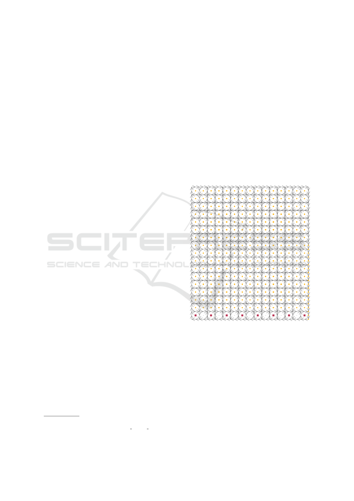
are 35x31 and 103x103, respectively. The directed

version of the warehouse design for Experiment 1 is

depicted in Figure 4 to show how the highways are

oriented.

Figure 4: Warehouse design for Experiment 1 with 17x15

building blocks.

For evaluation of another approach of warehouse

design, we prepared Experiment 3. The underlying

graph is depicted in Figure 5. To avoid agents block-

ing each others route to the extent that no agent can

make any movement, we needed to remove the hor-

izontal edges in the bottom of the graph as shown

in Figure 6. Again, only the directed version of the

CBSd algorithm is depicted in Figure 5. CBS was

evaluated on the same graph with the same edges, but

the edges were not oriented.

For all three warehouse designs, we initialized 100

random seeds to get 100 package destinations and run

ICAART 2022 - 14th International Conference on Agents and Artiﬁcial Intelligence

278

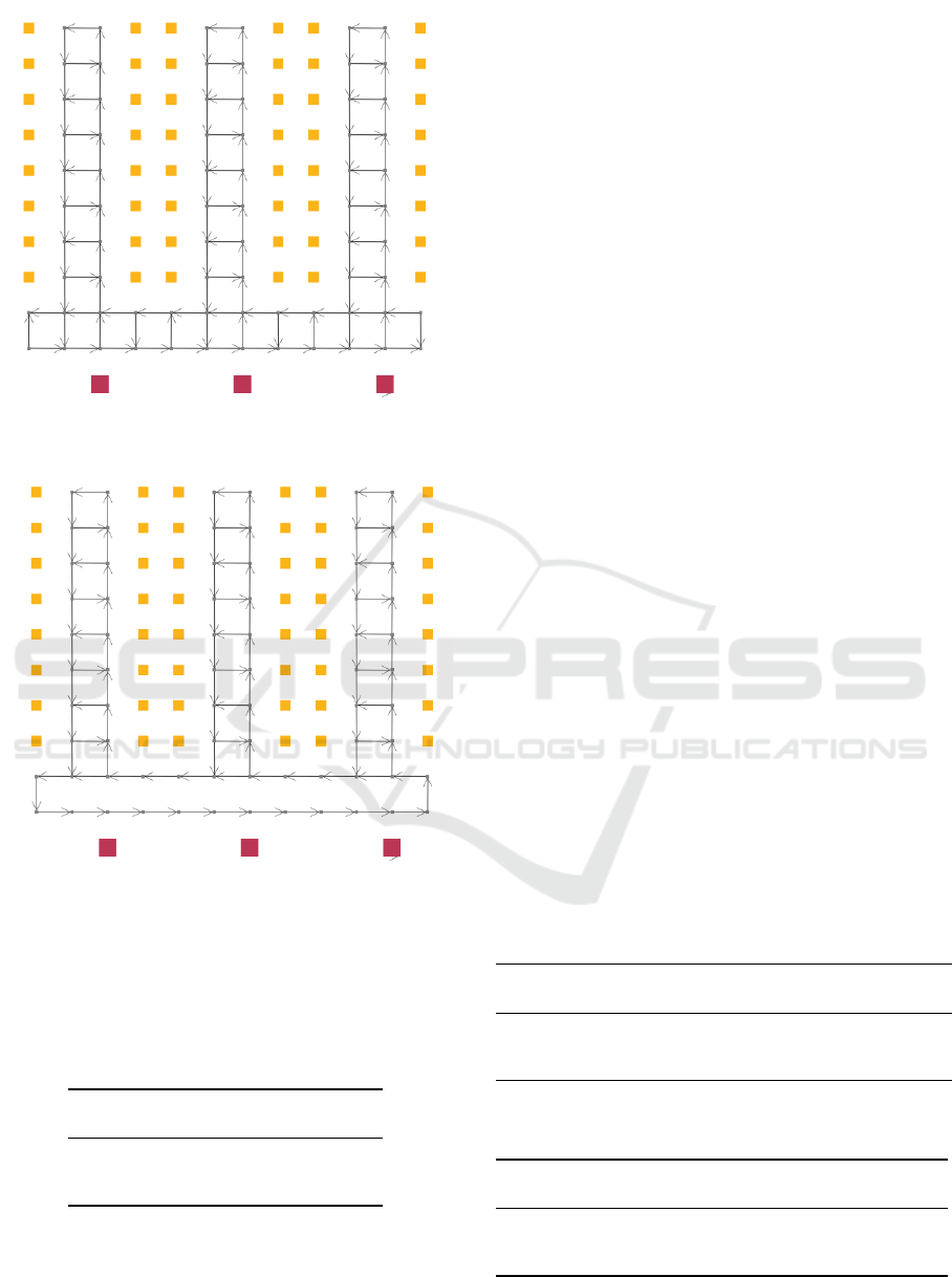
Figure 5: Warehouse design for Experiment 3 with CBS and

CBSd algorithms.

Figure 6: Warehouse design for Experiment 3 adjusted for

the Highway algorithm.

simulations to see how many time steps are needed to

deliver all packages to their designed locations.

Number of packages and sorting robots for each

of the experiments is show in Table 1.

Table 1: Experimental setup.

Experiment

number

Number of

packages

Number of

robots

1 300 60

2 1000 100

3 100 20

We used the following three planning strategies:

1. CBS on undirected graph,

2. CBS on directed graph,

3. HW on directed graph.

The last possible combination, HW on an undirected

graph, does not make sense as agents can easily block

each other with their planned moves.

At the time of unloading, the robot is given a new

destination which is a loading spot that has dispatched

the smallest number of packages until the present time

step.

Since an agent is given a new location every time

it loads or unloads a package, the CBS solver must be

called at every time step when a loading or unloading

action occurs to create a new collision-free plan.

Therefore, CBS algorithm only need to produce

a conﬂict-free plan for the smallest number of time

steps that are needed for any robot to reach its desti-

nation or a loading spot. Stopping CBS algorithm at

such a time step allows it to solve much complicated

problems compared to the case when CBS is required

to ﬁnd a conﬂict-free plan where all robots reach its

destinations.

4.3 Experimental Results

Results of the simulation runs described in the pre-

vious subsection are presented in Tables 2–4. In all

cases, all tracked parameters, i.e., minimal, maximal,

and average time span, CBS performs the best, fol-

lowed by CBS on a directed graph (CBSd) and HW.

To illustrate performance of the algorithms at ev-

ery time step we plot in Figures 7–9 how many pack-

ages had been delivered at each time step. Dim lines

presents the evolution of an simulation, bold lines

mean across all 100 simulations.

On the other hand, in case of Experiment 2 simu-

lations running on an average laptop, one simulation

run of HW takes, in general, about 0.05 second, CBSd

15 minutes, and CBS 1.5 hours.

Table 2: Times steps needed to deliver 300 packages in Ex-

periment 1.

Planning

Strategy

Min

Percentile

Max Mean Std

25 50 75

CBS 1107 1120 1130 1137 1158 1130 13

CBSd 1101 1130 1137 1146 1165 1137 13

HW 2167 2216 2234 2248 2313 2231 23

Table 3: Times steps needed to deliver 1000 packages in Ex-

periment 2.

Planning

Strategy

Min

Percentile

Max Mean Std

25 50 75

CBS 618 657 671 685 726 671 21

CBSd 634 676 689 709 738 690 23

HW 652 687 704 716 763 701 22

Highways in Warehouse Multi-Agent Path Finding: A Case Study

279

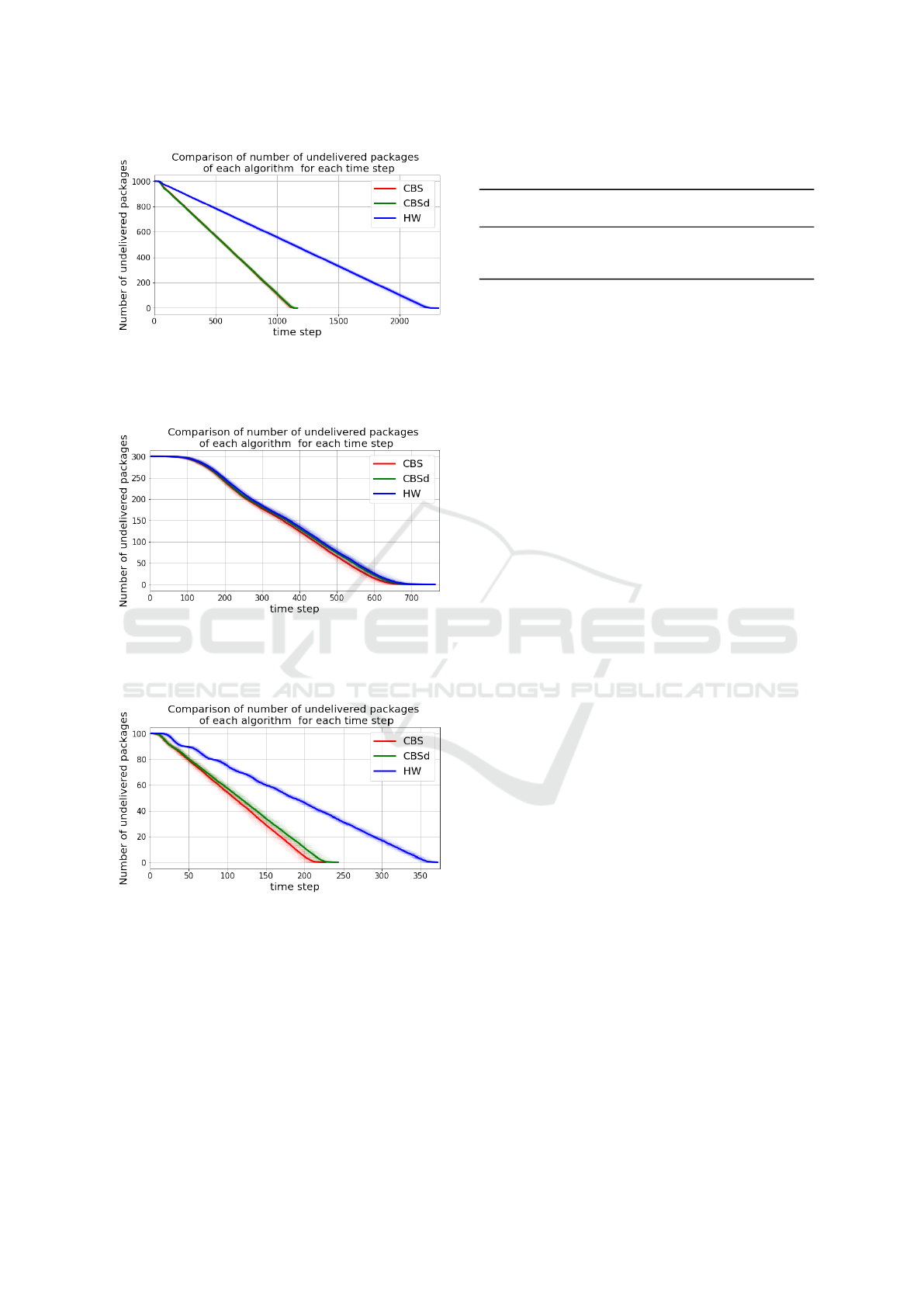
Figure 7: Mean of undelivered packages across all simula-

tions in Experiment 1. In this case the similar performance

of CBS and CBSd algorithms makes the red and green line

indistinguishable.

Figure 8: Mean of undelivered packages across all simula-

tions in Experiment 2. In this case the similar performance

of CBSd and Highway algorithms makes the green and blue

line indistinguishable.

Figure 9: Mean of undelivered packages across all simula-

tions for Experiment 3.

5 DISCUSSION

The results show that for Experiment 2, the average

difference in time needed to deliver 1000 packages

between a fast and simple algorithm and an optimal

one is about 5%.

A small difference between CBSd and HW might

suggest that the desired global conﬂict avoiding coor-

Table 4: Times steps needed to deliver 100 packages in Ex-

periment 3.

Planning

Strategy

Min

Percentile

Max Mean Std

25 50 75

CBS 194 205 210 215 227 209 7

CBSd 210 221 225 229 243 225 7

HW 349 356 359 364 372 360 6

dination is effectively introduced by imposing high-

ways in the graph.

Using CBS on the top of a directed graph im-

proves the average time span by 2-3 % while making

the simulation about 100 times slower.

With only about 5% difference in time span be-

tween a truly simple and fast algorithm and an optimal

one together with the rate by which every improve-

ment of the time span is prolonging the plan calcu-

lation, we conclude that it would be difﬁcult to beat

the HW algorithm while maintaining its computation

time.

The same conclusions would have been true for

Experiment 1 if we would have run simulations with

20 sorting robots. But when we employed 60 sorting

robots, the time span resulting from the HW algorithm

is twice as long as in the CBS or CBSd case. This

might suggest that HW is not particularly suited for

higher trafﬁc densities. Which turned to be true in the

last experiment as well.

In the case of Experiment 3, the difference in aver-

age time span is 7% between CBS and CBSd, but 70%

between CBS and HW. One would expect a difference

of such magnitude because route from the leftmost

loading spot the top left destination cage in the graph

in Figure 6 is more than twice as long as the route in

the graph in Figure 5. Carefully adding some of the

removed edges back to the graph depicted in Figure

6 could signiﬁcantly improve the performance of the

HW algorithm. Such an approach may need to take

into account the number of robots in the warehouse

graph.

Evaluation of the results and their application to

real-world scenarios make us believe that the most

frugal next step would be to focus on enriching our

warehouse abstraction model by incorporating as-

pects we neglected in this stage, described in Sec-

tion 3.

With the model taking into account robot accel-

eration/deceleration and turning as well as charging

needs we would like to discover whether in ware-

house model with suitable size the results from this

case study still holds. Then it might make sense to try

to answer questions such as how many robots in the

warehouse performs the best, which planning algo-

rithm is the most suitable one for a given scenario, or

ICAART 2022 - 14th International Conference on Agents and Artiﬁcial Intelligence

280

how to design a warehouse space to achieve maximal

warehouse sorting capacity.

ACKNOWLEDGEMENTS

The presented work has been supported by GA

CR -

the Czech Science Foundation under the grant regis-

tration number 22-31346S and by the Grant Agency

of the Czech Technical University in Prague, grant

registration number SGS20/213/OHK3/3T/18.

REFERENCES

Boyarski, E., Felner, A., Stern, R., Sharon, G., Tolpin,

D., Betzalel, O., and Shimony, S. E. (2015). ICBS:

improved conﬂict-based search algorithm for multi-

agent pathﬁnding. In Proceedings of the Twenty-

Fourth International Joint Conference on Artiﬁcial In-

telligence, IJCAI 2015, pages 740–746. AAAI Press.

Castiglione, F. (2009). Agent Based Modeling and Simula-

tion, Introduction to, pages 197–200. Springer New

York, New York, NY.

Cohen, L. and Koenig, S. (2016). Bounded suboptimal

multi-agent path ﬁnding using highways. In Kamb-

hampati, S., editor, Proceedings of the Twenty-Fifth

International Joint Conference on Artiﬁcial Intelli-

gence, IJCAI 2016, New York, NY, USA, 9-15 July

2016, pages 3978–3979. IJCAI/AAAI Press.

Datseris, G., Vahdati, A. R., and DuBois, T. C. (2021).

Agents.jl: A performant and feature-full agent based

modelling software of minimal code complexity.

Kautz, H. A. and Selman, B. (1999). Unifying sat-based

and graph-based planning. In Proceedings of the Six-

teenth International Joint Conference on Artiﬁcial In-

telligence, IJCAI 99, pages 318–325. Morgan Kauf-

mann.

Kornhauser, D., Miller, G. L., and Spirakis, P. G. (1984).

Coordinating pebble motion on graphs, the diame-

ter of permutation groups, and applications. In 25th

Annual Symposium on Foundations of Computer Sci-

ence, West Palm Beach, Florida, USA, 24-26 October

1984, pages 241–250. IEEE Computer Society.

Kornhauser, D., Wilensky, U., and Rand, W. (2009). De-

sign guidelines for agent based model visualization.

J. Artif. Soc. Soc. Simul., 12(2).

Lam, E., Bodic, P. L., Harabor, D. D., and Stuckey, P. J.

(2019). Branch-and-cut-and-price for multi-agent

pathﬁnding. In Proceedings of the Twenty-Eighth In-

ternational Joint Conference on Artiﬁcial Intelligence,

IJCAI 2019, pages 1289–1296. ijcai.org.

Ma, H., Tovey, C. A., Sharon, G., Kumar, T. K. S., and

Koenig, S. (2016). Multi-agent path ﬁnding with pay-

load transfers and the package-exchange robot-routing

problem. In Proceedings of the Thirtieth AAAI Con-

ference on Artiﬁcial Intelligence, 2016, pages 3166–

3173. AAAI Press.

Ryan, M. R. K. (2007). Graph decomposition for efﬁcient

multi-robot path planning. In IJCAI 2007, Proceed-

ings of the 20th International Joint Conference on Ar-

tiﬁcial Intelligence, pages 2003–2008.

Sharon, G., Stern, R., Felner, A., and Sturtevant, N.

(2015a). Conﬂict-based search for optimal multi-

agent pathﬁnding. Artif. Intell., 219:40–66.

Sharon, G., Stern, R., Felner, A., and Sturtevant, N. R.

(2015b). Conﬂict-based search for optimal multi-

agent pathﬁnding. Artif. Intell., 219:40–66.

Sharon, G., Stern, R., Goldenberg, M., and Felner, A.

(2013). The increasing cost tree search for optimal

multi-agent pathﬁnding. Artif. Intell., 195:470–495.

Silver, D. (2005). Cooperative pathﬁnding. In Proceedings

of the First Artiﬁcial Intelligence and Interactive Dig-

ital Entertainment Conference, pages 117–122. AAAI

Press.

Surynek, P. (2009). A novel approach to path planning

for multiple robots in bi-connected graphs. In 2009

IEEE International Conference on Robotics and Au-

tomation, ICRA 2009, Kobe, Japan, May 12-17, 2009,

pages 3613–3619. IEEE.

Surynek, P. (2010). An optimization variant of multi-robot

path planning is intractable. In Proceedings of the

Twenty-Fourth AAAI Conference on Artiﬁcial Intelli-

gence, AAAI 2010, Atlanta, Georgia, USA, July 11-15,

2010. AAAI Press.

Surynek, P. (2019). Unifying search-based and

compilation-based approaches to multi-agent path

ﬁnding through satisﬁability modulo theories. In

Kraus, S., editor, Proceedings of the Twenty-Eighth

International Joint Conference on Artiﬁcial Intelli-

gence, IJCAI 2019, pages 1177–1183. ijcai.org.

Surynek, P., Felner, A., Stern, R., and Boyarski, E. (2016).

Efﬁcient SAT approach to multi-agent path ﬁnding un-

der the sum of costs objective. In ECAI 2016 - 22nd

European Conference on Artiﬁcial Intelligence, vol-

ume 285 of Frontiers in Artiﬁcial Intelligence and Ap-

plications, pages 810–818. IOS Press.

Wurman, P., D’Andrea, R., and Mountz, M. (2008). Coordi-

nating hundreds of cooperative, autonomous vehicles

in warehouses. AI Magazine, 29:9–20.

Yu, J. and LaValle, S. M. (2013). Structure and intractability

of optimal multi-robot path planning on graphs. In

Proceedings of the Twenty-Seventh AAAI Conference

on Artiﬁcial Intelligence, July 14-18, 2013, Bellevue,

Washington, USA. AAAI Press.

Highways in Warehouse Multi-Agent Path Finding: A Case Study

281