Multi-agent Policy Gradient Algorithms for Cyber-physical Systems with

Lossy Communication

Adrian Redder

1 a

, Arunselvan Ramaswamy

1 b

and Holger Karl

2 c

Department of Computer Science, Paderborn University, Germany

Hasso-Plattner-Institute, Potsdam University, Germany

Keywords:

Policy Gradient Algorithms, Multi-agent Learning, Communication Networks, Distributed Optimisation,

Age of Information, Continuous Control.

Abstract:

Distributed online learning over delaying communication networks is a fundamental problem in multi-agent

learning, since the convergence behaviour of interacting agents is distorted by their delayed communication.

It is a priori unclear, how much communication delay can be allowed, such that the joint policies of multiple

agents can still converge to a solution of a multi-agent learning problem. In this work, we present the decen-

tralization of the well known deep deterministic policy gradient algorithm using a communication network.

We illustrate the convergence of the algorithm and the effect of lossy communication on the rate of conver-

gence for a two-agent ﬂow control problem, where the agents exchange their local information over a delaying

wireless network. Finally, we discuss theoretical implications for this algorithm using recent advances in the

theory of age of information and deep reinforcement learning.

1 INTRODUCTION

Centralized learning algorithms can usually be ex-

tended in a natural way to decentralized settings by

replacing global information with information that

has been communicated over a network. However,

the communication network typically induces infor-

mation delay, such that a centralized algorithm effec-

tively uses data that has a certain age of information

(AoI). In (Redder et al., 2021) practically veriﬁable

sufﬁcient conditions were presented, such that the AoI

associated with data communicated over graph based

networks behaves so that convergence of a distributed

stochastic gradient descend scheme can be guaran-

teed.

In this paper, we go one step further and consider a

multi-agent learning setting, where distributed agents

seek to ﬁnd local policies to solve a global learn-

ing problem. Speciﬁcally, we consider a multi-agent

learning algorithm, where agents update their local

policies conditioned on the policies of other agents

with a certain AoI, i.e. policies that the other agents

have used in the past.

https://orcid.org/0000-0001-7391-4688

https://orcid.org/0000-0002-8343-6322

https://orcid.org/0000-0001-7547-8111

Reinforcement learning (RL) problems pose addi-

tional challenges compared to stochastic optimisation

problems. In RL one typically optimizes a policy in

an online manner, where the interaction of the pol-

icy with an environment generates the observations

from the environment. In stochastic optimisation on

the other hand, one usually obtains observations of

an environment that are independent from the optimi-

sation variables of the problem. However, it was re-

cently shown that the convergence of many RL algo-

rithms can be analysed analogously to stochastic, iter-

ative gradient descend algorithms (Ramaswamy et al.,

2020). A natural question that therefore arises is,

whether one can decentralize, with the help of com-

munication, traditionally central RL algorithms to a

multi-agent setting without losing asymptotic conver-

gence guarantees.

In this paper, we therefore consider the decen-

tralization of the deep deterministic policy gradient

(DDPG) algorithm (Lillicrap et al., 2016) for the

multi-agent learning setting. We achieve this, by al-

lowing that the agents can frequently exchange their

current local policy and their local state-action pairs

over a communication network. At each local agent,

training is then performed by conditioning a policy

gradient step on the most recent available policy of

the other agents. For the communication network, we

282

Redder, A., Ramaswamy, A. and Karl, H.

Multi-agent Policy Gradient Algorithms for Cyber-physical Systems with Lossy Communication.

DOI: 10.5220/0010845400003116

In Proceedings of the 14th International Conference on Agents and Artiﬁcial Intelligence (ICAART 2022) - Volume 1, pages 282-289

ISBN: 978-989-758-547-0; ISSN: 2184-433X

present a simple illustrative model and present asso-

ciated conditions. We then show theoretically for this

model, that the effect of lossy communication on the

multi-agent learning algorithm will vanish asymptot-

ically. Therefore, asymptotic guarantees for the algo-

rithm with and without communication will be iden-

tical. Moreover, we also show that inﬁnitely many

global state-action pairs, will reach each agent.

We apply our algorithm to a simple but illustrative

two-agent water ﬁlter ﬂow control problem, where

two agents have to control the in- and outﬂow to wa-

ter ﬁlter. The agents have no information about the

dynamics of the ﬂow problem and have no prior in-

formation of the strategy of the other agents. But, the

agents are allowed to communicate over a network,

which therefore enables the use of our algorithm. Our

simulations show how the communication network

inﬂuences the rate of convergence of our multi-agent

algorithm.

2 BACKGROUND ON RL IN

CONTINUOUS ACTION SPACES

In this section we recall preliminaries on RL in con-

tinuous action spaces. In RL an agent interacts with

an environment E that is modeled as a Markov deci-

sion process (MDP) with state space S , action space

A, Markov transition kernel P, scalar reward func-

tion r(s,a). It does so by taking actions via a policy

µ : S → A. The most common objective in RL is to

maximize the discounted inﬁnite horizon return R

∑

∞

t=n

r(s

) with discount factor α ∈ [0,1). The as-

sociated action-value function is deﬁned as Q(s, a) =

µ,E

| s

= s,a

= 1]. The optimal action-value

function is characterized by the solution of the Bell-

man equation

∗

(s,a) = E



r(s, a) + α max

∈A

∗

)



s,a



(1)

Q-learning with function approximation seeks to ap-

proximate Q

∗

by a parametrized function Q(s,a; θ)

with parameters θ. For an observed tuple (s,a,r,s

this can be done by performing a gradient descent step

to minimize the squared Bellman loss



Q(s,a, ; θ) −(r(s, a) + α max

∈A

Q(s

;θ))



(2)

When the action space A is discrete, π(s) =

argmax

a∈A

Q(s,a; θ), ∀s ∈ S deﬁnes a greedy policy

with respect to Q(s,a,; θ). When A is continuous this

is not possible, but instead we can use Q(s, a; θ) to im-

prove a parametrized policy µ(s;φ) by taking gradient

steps in the direction of policy improvement with re-

spect to the Q-function:

∇

µ(s;φ)∇

Q(s,a; θ)|

a=µ(s;φ)

(3)

In (Silver et al., 2014) it was shown that the expec-

tation of (3) w.r.t the discounted state distribution in-

duced by a behaviour policy

is indeed the gradient of

the expected return of the policy µ. In practice, how-

ever, we usually do not sample from this discounted

state distribution (Nota and Thomas, 2020), but still

use (3) with samples from the history of interaction.

When the parametrized functions in (2) and (3) are

deep neural networks the corresponding algorithm is

then known as the deep deterministic policy gradient

algorithm (DDPG) (Lillicrap et al., 2016).

3 DECENTRALIZED POLICY

GRADIENT ALGORITHM

This section describes the adaptation of the DDPG al-

gorithm to the decentralized multi-agent setting.

3.1 Two-agent DDPG with Delayed

Communication

To simplify the presentation, we consider only two

agents 1 and 2. Consider an MDP as deﬁned in the

previous section and assume that agent 1 and 2 have

local action spaces A

and A

, respectively, such that

A = A

×A

is the global action space. Further, both

agents can observe local state trajectories s

∈ S

and

∈S

, such that S = S

×S

is the global state space.

Finally, we consider a global reward signal r

at every

time step n ≥ 0 that is observable by both agents.

The objective is that the agents learn local policies

;φ

) and µ

;φ

) parametrized by φ

and φ

maximize the accumulated discounted reward. The

global policy is therefore given by µ = (µ

,µ

). We

propose to use the DDPG algorithm locally at every

agent to train the policies µ

and µ

. However, to exe-

cute the DDPG algorithm locally, each agent requires

access to the parameters φ

and φ

at every time step

n ≥ 0. These parameter vectors are inherent local in-

formation of the agents and therefore are not a priori

available at the corresponding other agent.

Let us therefore suppose that the agents use a com-

munication network to exchange φ

and φ

. Since

communication networks typically induce informa-

tion delays, only φ

n−τ

(n)

and φ

n−τ

(n)

are available

at agent 1 and 2, respectively. Here, τ

(n) denotes the

The behaviour policy is typically µ distorted by a noise

process to encourage exploration.

Multi-agent Policy Gradient Algorithms for Cyber-physical Systems with Lossy Communication

283

AoI of φ

n−τ

(n)

at agent 1 at every time step n ≥ 0.

We refer to τ

(n) and τ

(n) as the AoI random vari-

ables variables. The communication network will be

discussed in the next section.

Let

= φ

n−τ

(n)

denote the latest available

parameter vector of agent 2 at agent 1. Sup-

pose, that agent 1 has access to a local approxima-

tion Q

(s,a; θ

) of the optimal Q-function Q

∗

(s,a)

parametrized by θ

at time n. Further, suppose the

agent can sample a realization of the global state

s = (s

). Then, at time n ≥ 0, agent 1 can calcu-

late a local policy gradient with respect to Q

that is

conditioned on the latest available policy of agent 2:

∇

;φ

)∇

(s,a; θ

)



s=s,a

=µ

;φ

),a

=µ(s

;

)

(4)

Equation (4) is therefore the φ

component (3),

where φ

is replaced by φ

n−τ

(n)

. In Algorithm 1,

we use this policy gradient to train the local policy

at agent 1. The algorithm of agent 2 is deﬁned anal-

ogously. We let both agents train its own local Q-

function using Deep Q-Learning. The agents might

also cooperate to ﬁnd better approximations of the Q-

function (Mnih et al., 2016). Observe that Algorithm

1 requires complete global tuples (s, a, r, s

) to execute

the training steps. We therefore assume that the agents

exchange their local states and actions over the com-

munication network in addition to their local policy

parametrizations. Ones a complete tuple is available,

each agent stores it in a local replay memory. Then

the local Q-function and local policy is updated using

sampled batches from the replay memory.

We would like to point out that the difference com-

pared to the central DDPG algorithm (Lillicrap et al.,

2016) is that the Bellman loss gradient in line 12 and

the policy gradient in line 13 of the algorithm take

into account the most recent available parametrisation

of the policy of agent 2. This implies that depending

to this parametrization, i.e. the expected behaviour

of agent 2, agent 1 will update its Q-function and its

policy differently. For completeness, one should add

target networks to the algorithm, since they are an im-

portant ingredient to stabilize RL with neural network

function approximators (Lillicrap et al., 2016).

3.2 Wireless Network Environment

Recall that Algorithm 1 requires that the agents do

exchange their policy parameters φ

as well as their

local information (s

), respectively. In this section

we describe a simple network environment used by

the two agents to exchange this information.

We represent the channel between the agents by

Algorithm 1: Algorithm at agent 1.

1 Randomly initialize critic and actor weights ;

2 Initialize replay memory R ;

3 for the entire duration do

4 Observe the current state s

;

5 Execute action a

= µ

;φ

) ;

6 Allocate s

and θ

for transmission to

agent 2 ;

7 Exchange data with agent 2 ;

8 Store new tuples (s,a,r,s

) in R ;

9 Sample a random batch of transitions

l+1

) from R ;

10 Compute targets y

= r

αQ

l+1

,µ

l+1

;φ

),µ

l+1

;

);θ

) ;

11 Update critic to minimize

;θ

) −y

)

averaged over the

sampled batch ;

12 Update µ

using (4) averaged over the

sampled batch ;

13 end

a signal-to-interference-plus-noise-ratio (SINR) mod-

els

SINR

, SINR

. (5)

At agent 1, SINR

is the instantaneous SINR of a re-

ceived signal transmitted with power p

during time

slot n by agent 2; I

is the experienced interference-

noise power during time slot n with some unknown,

but stationary distribution. For a time slot n, we as-

sume that SINR

and SINR

are constant. Given

SINR

in (5), we assume an SINR-threshold β such

that whenever the event A

= {SINR

1,n

≥ β} occurs

a transmission from node 2 to 1 can be successfully

received; hence, errors are due to interference. The

event A

is deﬁned analogously. The threshold β de-

pends on the modulation, coding and path character-

istics associated with each agent. The effective bit

rate R for the event A

is constraint by then Shannon

bounded R < B log

(1 + β) for a given bandwidth B.

Observe that typically the dimension of φ

is sig-

niﬁcantly larger that the dimension of (s

), since

the number of parameters of a function approxima-

tor (e.g. neural networks) would have to be increased

to allow better approximation as the dimension of

) increases. Lets assume that dim(φ) = d

and

that dim((s

)) = d

, with d

>> d

Now, observe that we are only interested in the

most recent φ

, while for training of the actor-critic

algorithm we can use all samples (s

). Therefore,

since d

>> d

, we may instead of transmitting a sin-

gle update for φ

transmit a large number of samples

). However, its unclear how we should weight

ICAART 2022 - 14th International Conference on Agents and Artiﬁcial Intelligence

284

the two data transmissions. For example, if d

≈ kd

for some k ≥ 0 we could transmit k samples after ev-

ery transmission of some φ

and therefore give equal

bandwidth usage to both. However, we may ﬁx any

ratio independent of d

and d

We now consider the following communication

protocol: Every agent keeps a backlog of samples that

have not been transmitted to the other agent. Then,

each agent transmits up to k ≥ 0 samples after every

complete transmission of its policy. Note that mul-

tiple events A

might need to occur to exchange all

components of some φ

, since d

is potentially large.

However, notice that the required number of events

is ﬁxed and determined by d

and d

, the used cod-

ing scheme and the effective bit rate R. The follow-

ing lemma shows that under suitable conditions the

AoI variables τ

(n) and τ

(n) grow asymptotically

slower than

√

n. Moreover, it shows that inﬁnitely

many global tuples reach each agent.

Lemma 1 . Suppose that p

> E [I

]β, p

> E [I

]β

and that the events A

are i.i.d., then we have that



(n) >

√

n inﬁnitely often



= 0 (6)

for both i ∈ {1,2}. Moreover, there is sequence

}

k≥0

, such that all samples (s

) have been re-

ceived at agent i.

Proof. It follows from p

> E [I

]β, p

> E [I

]β and

(Redder et al., 2021, Lemma 3) that P ((A

)

) > ε, for

some ε > 0. Here, (A

)

denotes the complement of

. Recall, that a ﬁxed ﬁnite number of events A

guarantees successful exchange of some φ

. Let l ≥

0 be the required number of events. Using that the

events A

are i.i.d., tt can then be shown that

P (τ

(n) > m) ≤Cε

, (7)

with some constant c independent of n and m. It fol-

lows that all τ

(n) are stochastically dominated by a

random variable with ﬁnite second moment, which

implies (6) using the Borel-Cantelli Lemma. In then

follows from (6) that there exists a sample path depen-

dent constant N, such that τ

(n) ≤

√

n for n ≥ N.

Remark 1 . For Lemma 1 we considered that the

interference-noise processes are stationary. How-

ever, one may also assume that the processes are

non-stationary, but instead that one is able to track

the processes mean asymptotically up some error

c ≥ 0. Then, assume p

> (E [I

] + c)β and p

(E [I

] + c)β in Lemma 1. Furthermore, it is sufﬁcient

that these conditions hold merely periodically or with

some positive probability. Then the agents may use an

arbitrary medium access and power scheduling pro-

tocol at all other time instances. Finally, the i.i.d. as-

sumption in Lemma 1 can be weakened to merely ex-

ponential dependency decay as discussed in (Redder

et al., 2021), or even more generally to dependency

decay with certain summability properties.

3.3 Theoretical Implication of Lemma 1

A detailed theoretical analysis of Algorithm 1 is out

of the scope for this work. However, we would like to

explain the use Lemma 1.

Consider Algorithm 1, where policies and Q-

functions are approximated by feed forward neural

networks. It was recently shown in (Ramaswamy and

Hullermeier, 2021) that for a large class of activa-

tion functions, including the Gaussian error linear unit

(GELU), the gradient of the neural network with re-

spect to its parameters is locally Lipschitz continuous

in the parameter coordinate. Hence, ∇

(s;φ

) is

locally Lipschitz in the φ

coordinate.

Suppose that φ

is updated with a decreasing step

size sequence γ(n) with

∑

n≥0

γ(n) = ∞,

∑

n≥0

γ(n)

∞. Further, suppose that Algorithm 1 is stable, i.e.

sup

n≥0

kφ

k< ∞ a.s. and sup

n≥0

k< ∞ a.s. Stability

of the algorithm iterates can be enforced by projecting

the iterates to sufﬁciently large compact set after each

update. The stability of the state trajectory can be re-

laxed to non-compact sets like R

see (Ramaswamy

and Hullermeier, 2021).

Under these assumptions, we can restrict our at-

tention to a compact set, where ∇

(s;φ

) is Lips-

chitz continuous in φ

. One can then show that the er-

ror in Algorithm 1, when considering θ

n−τ

(n)

instead

of θ

, satisﬁes

∈ o(γ(n)τ

(n)). (8)

It now follows from the assumption that γ is decreas-

ing with

∑

n≥0

γ(n)

< ∞ that γ(n) ∈ o(

√

n). Using

Lemma 1 we have that τ

(n) ≤

(n) for n ≥ N and a

sample bath dependent N ≥0. It therefore follows that

vanishes asymptotically. Hence, Algorithm 1 with

and without lossy communication behaves asymptot-

ically identical.

4 MULTI-AGENT

REINFORCEMENT LEARNING

FOR FLOW CONTROL

In this section we introduce a two-agent ﬂow control

problem to illustrate the use of Algorithm 1. Flow

control is an important problem in chemical indus-

tries, data centre cooling and water treatment plants.

In our two-agent example each agent has to control

one valve of a ﬂow control problem. Speciﬁcally, we

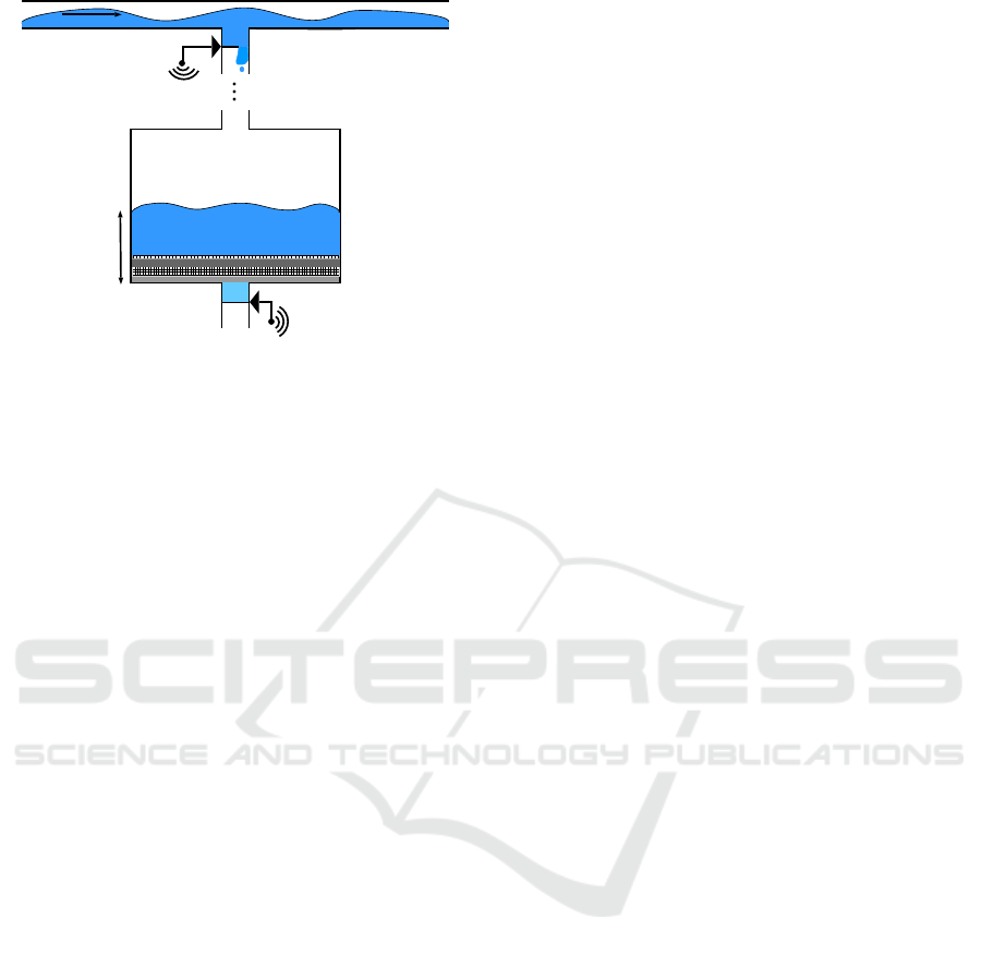
consider the water ﬁlter in Figure 1.

Multi-agent Policy Gradient Algorithms for Cyber-physical Systems with Lossy Communication

285

Agent 1

Agent 2

Figure 1: Illustration of the two agent water ﬁlter ﬂow con-

trol problem.

4.1 Water Filter Flow Control Problem

In Figure 1 agent 1 has to control the inﬂow to the

water ﬁlter from a main water line using valve a

Agent 2 has to control the outﬂow of the water ﬁl-

ter using valve a

. We consider that time is slotted

into small intervals of constant length ∆. The discrete

time steps are indexed by n ∈ N. We refer to a time

slot n as the time interval from time step n −1 to n.

For both agents, we consider that the valves can be

positioned continuously from close to open. There-

fore, at every time step n the agents have to pick ac-

tions a

∈ [0,1] for the associated time slot n. For

every time slot n, we denote the sampled ﬂow in the

main line by s

∈ S

⊂ R

≥0

and the sampled water

level in the water ﬁlter by s

∈ S

⊂ R

≥0

. The prob-

lem is complicated, since the agents have no informa-

tion about the dynamics of the main water line and

the water ﬁlter. Additionally, the agents have no in-

formation about the policy of the other agent, i.e. the

agents initially have no information about the strat-

egy of the other agent to control its valve. However,

we assume that the agents can use a wireless network

to exchange information, which therefore enables the

use of Algorithm 1.

Given s

and a

for some time step n, we assume

a continuous function f (s

) that determines the in-

ﬂow to the ﬁlter during time slot n. Equivalently, we

can assume that agent 1 can measure the inﬂow to

the ﬁlter. Other than that we make no additional as-

sumptions. The agents have no information about the

dynamics of the ﬁlter or of the ﬂow in the main water

line. We consider that the agents have to learn how to

control the valves solely based on their local actions,

observations and the information communicated with

the other agent.

4.2 Partial Observability Issues

Algorithm 1 formulates a decentralized multi-agent

solution based on locally observed states. The train-

ing procedure, however, can use delayed global infor-

mation that has been communicated over a network.

The solution therefore falls under the paradigm of de-

centralized training with central data, but decentral-

ized execution. Depending on how the local state

spaces are deﬁned, agents may or may not be able to

ﬁnd good solutions for a problem, since the local poli-

cies should only use local states, such that inference

is decentralized.

Now consider the ﬂow control problem of the pre-

vious subsection. If agent 1 can only observe the state

and never state s

, then it can only learn to take

very conservative actions, since it has no information

about the current amount of water in the water ﬁlter.

We expect better solutions, if both agents can observe

the whole state space s = (s

). A system theoretic

solution to this would now be to utilize a suitable local

estimator and replace s

by an estimate ˆs

at agent 1to

execute a local policy that is functions of the global

state space. Alternative, one could directly replace s

by its delayed counterpart and utilize a recurrent ar-

chitecture for the policies µ

and µ

, see for example

(Hausknecht and Stone, 2015).

Since our objective with this example is to illus-

trate the effect of lossy communication on the learn-

ing algorithm and not the effect on the quality infer-

ence, we assume here for simplicity that both agents

can observe s

and s

. Below, we therefore formu-

late the MDP for the two-agent ﬂow control problem,

where both agents observe s = (s

). Moreover, the

agents therefore only need to communicate their local

actions a

and a

, as well as their policy parametriza-

tions φ

and φ

4.3 An MDP for Two-agent Flow

Control

We consider the following high-level objective for the

two-agent ﬂow control problem:

(i) Maximize the through ﬂow of the ﬁlter.

(ii) Avoid under- and overﬂows, i.e. 0 < s

< 1 for

all n ≥ 0.

(iii) Try to keep a reserve of s

≈ 1/2 as good as

possible for all n ≥ 0.

The state space for both agents is deﬁned as S

1,2

×S

. The action spaces are deﬁned as A

= [0,1]

and A

= [0,1], respectively. To achieve the for-

mulated objective, we consider a continuous reward

ICAART 2022 - 14th International Conference on Agents and Artiﬁcial Intelligence

286

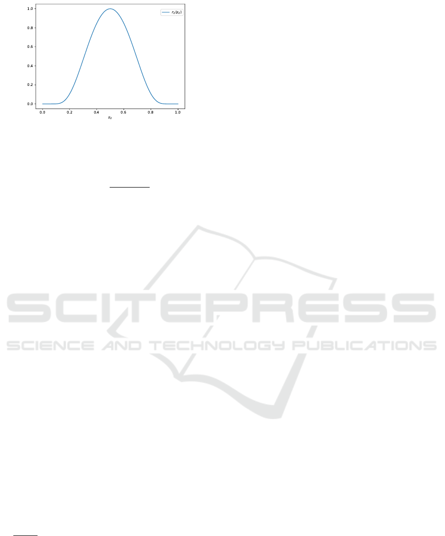
Figure 2: Plot of the second component, r

), of the re-

ward function.

function r(s

) = f (s

)c + r

), with

) = exp



(2s

−1)

−1)s



, (9)

and some constant c > 0 that may be used to weight

the importance of (i) over (ii) and (iii). Recall that f

is the function that determines the inﬂow to the wa-

ter ﬁlter. The inﬂow can also be measured by agent 1

and communicated to agent 2 alongside a

, since the

reward is also only required for training and not for in-

ference. Figure 2 shows the second component of the

reward function. We choose this function to satisfy

point (ii) and (iii) of our objective. Clearly, various

other shapes for the reward function are possible.

5 NURMERICAL SIMULATION

In this section, we present the numerical evaluation of

Algorithm 1 for the water ﬂow control MDP of Sec-

tion 4.3. Our goal is to illustrate the convergence of

our algorithm while the two agents communicate over

a lossy communication network. Most importantly,

we illustrate for this example how the lossy commu-

nication inﬂuences the rate of convergence of Algo-

rithm 1.

5.1 System and Algorithm Model

For our simulation we consider the following differ-

ential equation

(t)

−K

(t)a

(t)+K

(ρgs

(t))a

(t) = 0 (10)

to model the water ﬁlter. Here A is the area of the

water ﬁlter, ρ is the density of water, g the accel-

eration of mass, and K

and K

are constants. The

factor ρgs

(t) is the so called differential pressure at

time t (Rossiter, 2021). The second term is a bilin-

ear model for the inﬂow of the system. The third

term is a bilinear model for the outﬂow of the ﬁl-

ter. The constant K

includes the resistance of the

ﬁlter and the resistance of the outﬂow pipe. This is

only an approximate model for “small” changes of

the ﬂow. However, it serves the purpose for our eval-

uation. For our simulation, we solve equation (10)

numerically for time slots n of length ∆ = 1s, where

we assume that s

and s

are approximately constant

over each time slot. The agents then observe the sam-

ple of s

= (s

) from the beginning of each time

slot. For the constants in eq. (10), we use K

= 0.1,

which corresponds to a maximum inﬂow of 10% of

the main ﬂow, and K

= 10

−5

, which models the high

resistance of the water ﬁlter. Finally, we use c = 0.1 to

give high weight to balancing the water ﬁlter around

/2.

For Algorithm 1, we use the following set of pa-

rameters: Both agents approximate the Q-function by

a two-layer neural network with 256 and 128 Gaus-

sian error linear units (GELU’s) as activation’s. The

ﬁnal single neuron output layer is linear layer. Both

policies µ

and µ

are also represented by two-layer

neural networks, where each layer has 64 GELU’s and

a tanh output layer. We use α = 0.95 and a training

batch size of 128. We also use target networks and

an Ornstein-Uhlenbeck noise process for exploration

(Lillicrap et al., 2016).

5.2 Network Model

To emulate a delaying communication network, we

merely consider two Bernoulli processes. We assume

that P (A

) = λ at every time step n for both agent 1

and 2. We then choose λ ∈ {1,

/2,

/4,

/8,

/16,

/32}.

Practically, this corresponds a suitable choice of the

power schedule p

and p

for given i.i.d. interference-

noise processes I

and I

. However, to make the com-

munication model more realistic, we assume a nar-

rowband wireless channel with B = 10Mhz and a typ-

ical choice β = 7. Then, we can obtain an effective

bitrate of 19

Mbit

/s. Now, suppose we code every real

number using 64 bits. Then, observe that each pol-

icy contains 4544 real-valued parameters and since

we merely require the exchange of the actions a

only need to exchange one real number to obtain a

sample (s

). Therefore, we require at least 16 time

slots of successful communication to transmit a single

policy update, while in each time slot we can transmit

more than 300 samples. For our experiments, we give

roughly equal bandwidth usage to the parameter- and

sample transmissions. Speciﬁcally, each agent trans-

mits a single update to its parameter vector followed

by the transmission of up to 300 ·16 samples or until

its backlog is empty.

Multi-agent Policy Gradient Algorithms for Cyber-physical Systems with Lossy Communication

287

Figure 3: Average reward after each training epoch.

5.3 Training

We train the agents over 500 epochs with length T =

100. The Q- and policy networks are updated with the

ADAM optimizer (Kingma and Ba, 2015) using Ten-

sorﬂow 2. We use the following learning rate sched-

ules

γ(n) =

−8

1000

+ 1

−7

−e

−8



1000

+ 1



, δ(n) =

−8

1000

+ 1

(11)

These learning rates satisfy the standard assumptions

from the stochastic approximation (SA) literature, i.e.

they are not summable, but square summable. More-

over, they satisfy

γ(n)

δ(n)

→ 1. Although non-standard

in the SA literature, this assumption enables the use

of tools developed in (Ramaswamy and Hullermeier,

2021) to show the convergence of Algorithm 1 (Red-

der et al., 2022).

Figure 3 shows the average reward at the end

of each training epoch evaluated without exploration

noise on a new trajectory of length T = 1000 for ev-

ery λ. Observe that for all λ the algorithm converges

to a policy of similar average reward compared to Al-

gorithm 1 without communication and global infor-

mation access. Moreover and as expected, as λ de-

creases the rate of convergence also decreases. How-

ever, for λ ∈ {1,

/2,

/4} the effect of lossy communi-

cation seams to be minor.

After training, we evaluated the ﬁnal policies on

a new trajectory. For illustration we show the results

for λ = 1/16. In Figure 4 we show the inﬂow to the

water ﬁlter, the water level in the ﬁlter and the re-

ward per step. In the water level plot, we see that

the agents learned to quickly balance the water level

around the desired height s

/2. The inﬂow is upper

bounded by the maximal possible inﬂow for a

= 1.

The reward per step is upper bounded by 1 plus the

aforementioned upper bound. However, the maximal

Figure 4: Main ﬂow, inﬂow and water level during one tra-

jectory after training.

Figure 5: Actions associated with the simulated trajectory

after training.

possible inﬂow and therefore the maximal possible re-

ward per step may not be obtainable, since opening

the inﬂow valve fully may lead to an increase of the

desired height even when the outﬂow valve is fully

opened. We can observe this between time step n = 50

to n = 400. For this, consider the associated actions

during the trajectory in Figure 5. We see that when

the inﬂow is to large in [50,400], agent 1 has to re-

duce the inﬂow to the system, while agent 2 has to

fully open the outﬂow. In this time interval the inﬂow

part of the reward becomes signiﬁcant and therefore

the agents learned to maximize the inﬂow.

We can also observe that for the second halve of

the trajectory the algorithm could potentially improve

with longer training. Here, the agents mainly balance

the water level at the desired height, since the inﬂow

is relatively small and since we chose c = 0.1. How-

ever, opening the inﬂow valve more can still lead to a

slightly larger reward per step. In summary, we have

seen that agents are able to learn non-trivial policies

for an unknown environment in the presence of highly

uncertain communication.

ICAART 2022 - 14th International Conference on Agents and Artiﬁcial Intelligence

288

6 CONCLUSIONS

We showed how the DDPG algorithm can be imple-

mented in a distributed, multi-agent scenario using a

communication network. We gave a theoretical dis-

cussion of the impact of the communication errors on

the learning algorithm and validated the convergence

of our algorithm for a two-agent example. For future

work, we are interested in a fully end-to-end learning

based solution, where agents use communicated, de-

layed state information as their local states. This can

be done using recurrent architectures for the policies

and µ

. The architecture would use the most recent

available state and its corresponding age. The objec-

tive is that the recurrent architecture internally pre-

dicts the true current state, and then selects an action

conditioned on the prediction error and the policy that

one would associate with global state observations.

ACKNOWLEDGEMENTS

Adrian Redder was supported by the German Re-

search Foundation (DFG) - 315248657 and SFB 901.

We would also like to thank Eva Graßkemper for cre-

ating Figure 4.

REFERENCES

Hausknecht, M. and Stone, P. (2015). Deep recurrent q-

learning for partially observable mdps. In 2015 aaai

fall symposium series.

Kingma, D. P. and Ba, J. (2015). Adam: A method for

stochastic optimization. In ICLR.

Lillicrap, T. P., Hunt, J. J., Pritzel, A., Heess, N., Erez, T.,

Tassa, Y., Silver, D., and Wierstra, D. (2016). Con-

tinuous control with deep reinforcement learning. In

ICLR (Poster).

Mnih, V., Badia, A. P., Mirza, M., Graves, A., Lillicrap, T.,

Harley, T., Silver, D., and Kavukcuoglu, K. (2016).

Asynchronous methods for deep reinforcement learn-

ing. In International conference on machine learning,

pages 1928–1937. PMLR.

Nota, C. and Thomas, P. S. (2020). Is the policy gradi-

ent a gradient? In Proceedings of the 19th Interna-

tional Conference on Autonomous Agents and Multi-

Agent Systems, pages 939–947.

Ramaswamy, A., Bhatnagar, S., and Quevedo, D. E. (2020).

Asynchronous stochastic approximations with asymp-

totically biased errors and deep multi-agent learning.

IEEE Transactions on Automatic Control.

Ramaswamy, A. and Hullermeier, E. (2021). Deep q-

learning: Theoretical insights from an asymptotic

analysis. IEEE Transactions on Artiﬁcial Intelligence.

Redder, A., Ramaswamy, A., and Karl, H. (2021). Prac-

tical sufﬁcient conditions for convergence of dis-

tributed optimisation algorithms over communica-

tion networks with interference. arXiv preprint

2105.04230.

Redder, A., Ramaswamy, A., and Karl, H. (2022). Asymp-

totic convergence of deep multi-agent actor-critic al-

gorithms. Under review for AAAI 2022.

Rossiter, A. (2021). Modelling, dynamics and con-

trol. https://controleducation.group.shef.ac.uk/

chaptermodelling.html. Accessed: 25.05.2021.

Silver, D., Lever, G., Heess, N., Degris, T., Wierstra, D., and

Riedmiller, M. (2014). Deterministic policy gradient

algorithms. In International conference on machine

learning, pages 387–395. PMLR.

Multi-agent Policy Gradient Algorithms for Cyber-physical Systems with Lossy Communication

289