Efﬁcient Multi-angle Audio-visual Speech Recognition using Parallel

WaveGAN based Scene Classiﬁer

Shinnosuke Isobe

1 a

, Satoshi Tamura

, Yuuto Gotoh

and Masaki Nose

Graduate School of Natural Science and Technology, Gifu University, Gifu, Japan

Faculty of Engineering, Gifu University, Gifu, Japan

Ricoh Company, Ltd., Kanagawa, Japan

Keywords:

Scene Classiﬁcation, Audio-visual Speech Recognition, Multi-angle Lipreading, Anomaly Detection, Neural

Vocoder.

Abstract:

Recently, Audio-Visual Speech Recognition (AVSR), one of robust Automatic Speech Recognition (ASR)

methods against acoustic noise, has been widely researched. AVSR combines ASR and Visual Speech Recog-

nition (VSR). Considering real applications, we need to develop VSR that can accept frontal and non-frontal

face images, and reduce computational time for image processing. In this paper, we propose an efﬁcient multi-

angle AVSR method using a Parallel-WaveGAN-based scene classiﬁer. The classiﬁer estimates whether given

speech data were recorded in clean or noisy environments. Multi-angle AVSR is conducted if our scene clas-

siﬁcation detected noisy environments to enhance the recognition accuracy, whereas only ASR is performed

if the classiﬁer predicts clean speech data to avoid the increase of processing time. We evaluated our frame-

work using two multi-angle audio-visual database: an English corpus OuluVS2 having 5 views and a Japanese

phrase corpus GAMVA consisting of 12 views. Experimental results show that the scene classiﬁer worked

well, and using multi-angle AVSR achieved higher recognition accuracy than ASR. In addition, our approach

could save processing time by switching recognizers according to noise condition.

1 INTRODUCTION

Recently, Automatic Speech Recognition (ASR) has

been conﬁrmed to have high recognition performance

by using Deep Learning (DL), one of artiﬁcial intel-

ligence (AI) techniques, and is used in various real

scenes such as voice input for mobile phones and

car navigation systems. However, there is a prob-

lem that speech waveforms are degraded by acoustic

noise in real environments, reducing the accuracy of

speech recognition. In order to overcome this issue,

we need to develop robust ASR systems against any

audio noise. One of such ASR systems applicable in

noisy environments is Audio Visual Speech Recogni-

tion (AVSR, also known as multimodal speech recog-

nition), which employs ASR frameworks with Visual

Speech Recognition (VSR, also known as lipreading).

VSR uses lip images which are not affected by audio

noise and estimates what a subject uttered only from

a temporal sequence of lip images. VSR and AVSR

have a potential to be applied in various practical ap-

https://orcid.org/0000-0002-7011-3081

plications such as automatic conference minute gen-

eration and human interface on smartphones. Owing

to state-of-the-art DL technology, recently we have

achieved high performance of VSR.

AVSR has been investigated mainly for a couple

of decades and improves speech recognition accuracy

signiﬁcantly. However, there are still several issues

remaining regarding VSR and AVSR. The ﬁrst one is

that a speaker does not always face to a camera such

as smart device or tablet device in real environments.

In other words, most of existing VSR and AVSR re-

search works have only considered frontal faces, al-

though VSR technology for non-frontal views is also

essential for real applications. The second issue is in-

creasing processing time. AVSR must conduct image

processing in addition to speech processing simul-

taneously, resulting larger computational costs than

ASR and VSR. In noisy environments, because AVSR

can drastically improve speech recognition accuracy,

it is worthy to carry out AVSR even if longer process-

ing time is required. On the other hand, in clean envi-

ronments, ASR and AVSR often have almost the same

and signiﬁcantly high recognition accuracy because

Isobe, S., Tamura, S., Gotoh, Y. and Nose, M.

Efﬁcient Multi-angle Audio-visual Speech Recognition using Parallel WaveGAN based Scene Classiﬁer.

DOI: 10.5220/0010846000003122

In Proceedings of the 11th International Conference on Pattern Recognition Applications and Methods (ICPRAM 2022), pages 449-460

ISBN: 978-989-758-549-4; ISSN: 2184-4313

449

speech signals are not polluted by acoustic noise. This

means that only applying ASR is sufﬁcient to obtain

acceptable speech recognition performance.

Regarding the ﬁrst problem, we have already de-

veloped a multi-angle VSR, which can accept not

only frontal but also diagonal or proﬁles face images

(S.Isobe et al., 2021c; S.Isobe et al., 2020; S.Isobe

et al., 2021d). Therefore, in this article we would like

to focus on the second problem about processing time.

The straightforward strategy to handle the issue is to

introduce a noise estimator or a scene classiﬁer; if the

estimator judges given audio data as a clean speech,

we simply perform only ASR to obtain recognition

results; otherwise, we start to carry out image pro-

cessing followed by running multi-angle AVSR.

In this work we choose an anomaly-detection-

based scene classiﬁer for this purpose. We usu-

ally adopt an anomalous sound detection approach in

which a classiﬁer is trained using only acoustically

clean utterance data. One of conventional schemes

for anomaly detection is to employ a reconstruction

model, such as Autoencoder (AE) and Variational Au-

toencoder (VAE). However, in this case it is consid-

ered that these models are not appropriate; it is hard

for AE and VAE to reconstruct data having com-

plicated structures like speech signals, and in fact,

our preliminary experiments show the reconstruction

hardly succeeded. Therefore, in this work, we employ

an anomaly-detection-based scene classiﬁer using a

Parallel WaveGAN architecture (R.Yamamoto et al.,

2020), which is one of neural vocoders. Once the

Parallel WaveGAN model can be built signiﬁcantly,

it can well generate clean speech signals, on the other

hand, cannot correctly generate utterance data con-

taminated by acoustic noise. Consequently, noisy

speech signals must have higher anomaly scores, and

can be easily discriminated from clean audio data.

We conducted evaluation experiments using two

databases for multi-angle AVSR: an open corpus

OuluVS2 (I.Anina et al., 2015) and a GAMVA

(S.Isobe et al., 2021a) database which was proposed

in our previous research. We employed our multi-

angle VSR method, in which several angle-speciﬁc

VSR models were simultaneously applied and in-

tegrated based on angle estimation results (S.Isobe

et al., 2021c). As an ASR model, a 2D Convolu-

tional Neural Network (2DCNN) was chosen; mel-

frequency spectrograms were given to the model.

Angle-speciﬁc VSR models each consisted of a

3DCNN, and Bidirectional Long Short-Term Mem-

ory (Bi-LSTM) was adopted as an angle estimation

model using facial feature points. Experimental re-

sults showed that our proposed multi-angle AVSR

method with the scene classiﬁer achieved higher

recognition accuracy than ASR only, and faster than

our previous multi-angle AVSR method.

The rest of this paper is organized as follows. In

Section 2, we brieﬂy review related works. Section

3 summarizes our proposed system. Section 4 in-

troduces a proposed scene classiﬁcation method, fol-

lowed by ASR, multi-angle AVSR, and angle estima-

tor in Section 5. Two multi-angle audio-visual cor-

pora, experimental setup, results, and discussion are

described in Section 6. Finally Section 7 concludes

this paper.

2 RELATED WORK

In this section, we brieﬂy introduce AVSR, multi-

angle VSR / AVSR, neural vocoder based Text-To-

Speech (TTS) and anomaly detection.

2.1 AVSR

Many research works have been conducted focusing

on AVSR. In this paper we would like to introduce

a couple of state-of-the-art works. An AVSR sys-

tem based on a recurrent-neural-network transducer

architecture was built in (T.Makino et al., 2019).

They evaluated the system using the LRS3-TED data

set, achieving high performance. In (P.Zhou et al.,

2019), the authors proposed a multimodal attention-

based method for AVSR, which could automati-

cally learn fused representations from both modal-

ities based on their importance. They employed

sequence-to-sequence architectures, and conﬁrmed

high recognition performance under both acoustically

clean and noisy conditions. Another AVSR system

using a transformer-based architecture was proposed

in (G.Paraskevopoulos et al., 2020). Experimental re-

sults show that on the How2 data set, the system rela-

tively improved word error rate over sub-word predic-

tion models. In (S.Isobe et al., 2021b), we proposed

an AVSR method based on Deep Canonical Correla-

tion Analysis (DCCA). DCCA consequently gener-

ates projections from two modalities into one com-

mon space, so that the correlation of projected vectors

could be maximized. We thus employed DCCA tech-

niques with audio and visual modalities to enhance

the robustness of ASR. As a result, we conﬁrmed

DCCA features of each modality can improve com-

pared to original features, and got better ASR results

in various noisy environments.

ICPRAM 2022 - 11th International Conference on Pattern Recognition Applications and Methods

450

2.2 Multi-view VSR / AVSR

S. Petridis et al. proposed an end-to-end multi-view

lipreading system based on Bi-LSTM networks in

(S.Petridis et al., 2018). The model simultaneously

extracted features directly from image pixels and per-

formed visual speech classiﬁcation from multi-angle

views. Experimental results demonstrated the com-

bination of frontal and proﬁle views improved ac-

curacy over the frontal view. In (A.Koumparoulis

and G.Potamianos, 2018), they proposed a scheme

called ”View2View” using an encoder-decoder model

based on CNNs. The method transformed non-frontal

mouth-region images into frontal ones. Their results

show that the view-mapping system worked well for

VSR and AVSR. In (S.Isobe et al., 2020), we pro-

posed a feature-integration-based multi-angle lipread-

ing system using DL, particularly 3DCNN, that is one

kind of Deep Neural Networks (DNNs).

In spite that we can ﬁnd a lot of VSR and AVSR

methods, there are only a few works combining ASR

and multi-angle VSR to accomplish angle-invariant

AVSR. One of them is (S.Petridis et al., 2017), where

they proposed an early-fusion-based AVSR method

using Bi-LSTMs. In our previous research works,

we also focused on multi-angle AVSR (S.Isobe et al.,

2021c; S.Isobe et al., 2021d). In (S.Isobe et al.,

2021c), we propose a new multi-angle lipreading

method, in which several angle-speciﬁc VSR models

are simultaneously performed and integrated based

on angle estimation results. In addition, we con-

ducted decision-fusion-based AVSR. Experimental

results show that our proposed method can accept

lip images at various angles, and improve the recog-

nition accuracy in noisy environments. In (S.Isobe

et al., 2021d), we further extended our previous VSR

to AVSR schemes (S.Isobe et al., 2020).

2.3 Neural Vocoder

In this paper, we select a Parallel WaveGAN model

as a neural vocoder. Nowadays several the other

neural vocoder methods have been proposed in ad-

dition to Parallel WaveGAN. Firstly, we introduce a

WaveNet model (A.Oord et al., 2016), which is an

auto-regressive sequence model that generates highly

real audio waveforms conditioned on auxiliary fea-

tures and previous samples. Next, in (K.Kumar et al.,

2019), they proposed a multi-scale GAN-based archi-

tecture for discriminators. (J.Kong et al., 2020) gener-

ates both efﬁcient and high-quality audio waveforms.

They focused on speech audio of which components

are sinusoidal signals with various periods. Through

experimental results they conﬁrmed that the model-

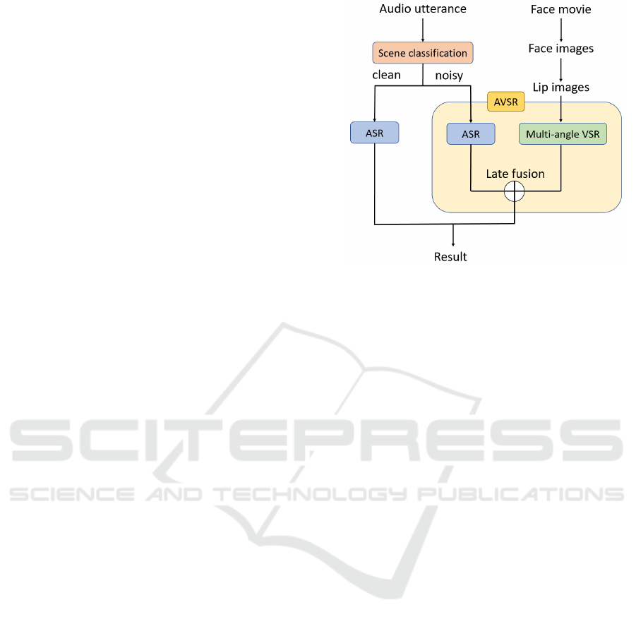
Figure 1: A ﬂow of our proposed method.

ing of periodic patterns of audio speeches is crucial

for enhancing sample quality.

2.4 Anomaly Detection

Finally, we introduced a few anomalous sound de-

tection research works. In (K.Suefusa et al., 2020),

they investigated conventional anomalous sound de-

tection methods based on the reconstruction errors,

and found that reconstruction models such as AE tend

to be large independent if the target sound is non-

stationary. To solve this problem, they adopted an ap-

proach in which the spectrograms of multiple frames

except their center frame were used as input, and the

deleted frame was predicted. If the model is built

using normal data, anomaly data cannot be well pre-

dicted. In (K.Inagaki et al., 2020), they extracted the

output of an intermediate layer of an AE, and calcu-

lated the degree of abnormality for the output based

on a Gaussian Mixture Model (GMM), representing

a data set by superposition of a mixture of Gaussian

distributions. Since many manufacturing companies

have great interests in anomaly detection, recently

competitions of anomalous sound detection such as

(Y.Koizumi et al., 2020) were held worldwide.

3 METHODOLOGY

The ﬂow of the proposed method is shown in Fig.

1. First of all, an audio utterance is given to our

scene classiﬁcation model to determine whether the

data is noisy or clean. If the utterance is classi-

ﬁed as clean speech, only ASR is performed to ob-

tain speech recognition results. Otherwise, a face

Efﬁcient Multi-angle Audio-visual Speech Recognition using Parallel WaveGAN based Scene Classiﬁer

451

movie is loaded to the system, followed by conduct-

ing multi-angle VSR. Before multi-angle VSR, the

recorded face movie was converted to a face image

sequence. Thereafter, we get 68 face feature points

from each face images using face-alignment (A.Bulat

and G.Tzimiropoulos, 2017), and the LF-ROI (lower

face region of interest) is cut out to obtain lip images.

After that, AVSR is carried out to acquire recogni-

tion results in the late-fusion manner. Our system ﬁ-

nally outputs either results from ASR or those from

AVSR according to scene classiﬁcation. Note that, if

the face feature points are not detected, we conducted

only ASR.

4 SCENE CLASSIFICATION

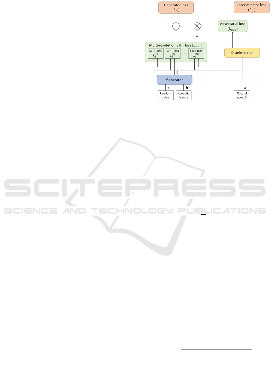
4.1 Parallel WaveGAN

Parallel WaveGAN is one of non-autoregressive neu-

ral vocoders, and one of the Generative Adversarial

Networks (GANs). The architecture of Palallel Wave-

GAN is shown in Fig. 2. GANs are generally cat-

egorized into generative models, having two neural

network models: a generator (G) and a discrimina-

tor (D). In the GAN framework, a generator tries

to create fake data which are almost the real one as

much as possible. A discriminator, on the other hand,

tries to classify fake and real data as correct as possi-

ble. Generator and discriminator are thus adversar-

ial, and trained so that either of them tries to fool

another model, ﬁnally resulting high-level generator

and discriminator. In the TTS ﬁeld, some of research

works have been reported to generate high-quality au-

dio waveforms using GANs. WaveNet (A.Oord et al.,

2016) is one of such the generative model that is of-

ten used in the ﬁeld. However, WaveNet has a short-

age that the processing speed is very slow, because the

model has an autoregressive architecture. In contrast,

Parallel WaveGAN is able to be trained and generate

data very fast, because of the parallel architecture.

4.1.1 Generator

The generator model is a WaveNet-based one, receiv-

ing acoustic features and random noise drawn from

a Gaussian distribution as input, and generating par-

allel audio waveforms. Causal convolutions are used

in WaveNet, while in Parallel WaveGAN they are re-

placed into non-causal convolutions.

Here we describe a generator loss function related

to the generator model. First, the generator loss L

can be computed as a linear combination of a multi-

resolution Short-Time Fourier Transform (STFT) loss

Figure 2: An overview of Parallel WaveGAN.

and an adversarial loss as follows:

(G, D) = L

aux

(G) + α L

adv

(G, D), (1)

where L

aux

and L

adv

are a multi-resolution STFT loss

and an adversarial loss, respectively. A hyperparame-

ter α in Equation 1 is used to balance two loss func-

tions. In this paper, α is set to 4.0 as in the original

paper. The multi-resolution STFT loss is a mean of

STFT loss values. Every STFT loss scores are ob-

tained in different Fast Fourier Transform (FFT) set-

tings, such as FFT size, window size, frame shift, and

so on. The multi-resolution STFT loss is then calcu-

lated as follows:

aux

(G) =

∑

m=1

(m)

(G), (2)

where L

(m)

is an m-th single STFT loss, and M is the

total number of STFT loss scores. There are two main

reasons for combining single STFT losses under sev-

eral conditions. The ﬁrst one is to prevent overﬁt-

ting to any ﬁxed STFT representation. Another rea-

son comes from a trade-off relationship between time

and frequency resolution. The generator model is

thereby able to learn the time-frequency characteris-

tics of speech data by combination several STFT loss.

The single STFT loss denotes by the following equa-

tion:

(G) = L

(x, ˆx) + L

mag

(x, ˆx), (3)

where x and ˆx are original data and generated data,

respectively. In Equation 3, L

and L

mag

are spectral

convergence and log STFT magnitude loss, respec-

tively:

(x, ˆx) =

|| |STFT(x)| − |STFT( ˆx)| ||

|| |STFT(x)| ||

, (4)

mag

(x, ˆx) =

|| log|STFT(x)| − log|STFT( ˆx)| ||

(5)

ICPRAM 2022 - 11th International Conference on Pattern Recognition Applications and Methods

452

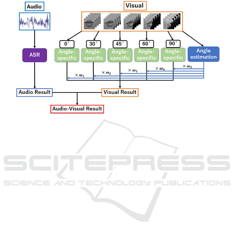
Figure 3: An overview of our AVSR method. This architecture is for OuluVS2, having ﬁve angle-speciﬁc VSRs.

where ||·||

, ||·||

, |STFT(·)| are Frobenius, L1 norm

and STFT magnitudes respectively, and N is number

of magnitude elements.

Second, the adversarial loss is deﬁned as follows:

adv

(G, D) = E

z∈N(0,I)

[(1 − D(G(z, h)))

], (6)

where z, N(0, I) and h are random noise drawn from

a Gaussian distribution, a Gaussian distribution with

zero mean and standard deviation of I, and condi-

tional acoustic feature (such as mel-frequency spec-

trogram), respectively. ˆx = G(z, h) indicates gener-

ated data, and 0 ≤ D(x) ≤ 1 means a classiﬁcation re-

sult. The adversarial loss is designed based on least-

squares GANs (X.Mao et al., 2017) for stable train-

ing.

4.1.2 Discriminator

The discriminator model consists of ten non-causal

dilated 1D convolution layers with the leaky ReLU

activation function (α = 0.2). The loss function for

the discriminator is shown below:

(G, D) =E

x∈p

data

[(1 − D(x))

]

+ E

z∈N(0,I)

[(1 − D(G(z, h)))

(7)

where p

data

is a target waveform distribution.

4.2 Parallel WaveGAN for Scene

Classiﬁcation

Here, we introduce how to classify whether a given

audio utterance is clean or noisy data using Parallel

WaveGAN. Firstly, we train Parallel WaveGAN using

only clean speech data. After that, we employ not the

discriminator but the generator for the purpose. Given

feature vectors of clean speech data which are not

used for model training, the generator model of Par-

allel WaveGAN is able to generate the corresponding

speech waveform correctly. That is, the model tries

to imitate the same speech signal from the given mel-

frequency spectrogram features. On the other hand,

taken noisy audio features with background noise, the

model cannot imitate the speech utterance correctly.

Hence, by comparing the original speech signal and

the generated speech signal from Parallel WaveGAN,

we can judge whether the input original signal con-

tains background noise or not, i.e. clean or noisy.

This is based on general unsupervised anomaly

sound detection using generation and reconstruction

model. AE and VAE are expected to work prop-

erly for audio signals having relatively simple struc-

tures such as machine operating acoustic data with

stationary anomaly sounds. However, because speech

signals are basically much more complicated, if we

choose the same strategy, deeper and larger AEs

might be needed for speech reconstruction, requir-

ing the huge amount of training data. We then think

employing the Parallel WaveGAN is smarter way for

speech data. Regarding loss functions, we conducted

preliminary experiments to measure a better anomaly

score function, and which loss function should be in-

volved for training. We then found that the multi-

resolution STFT loss function is better than the mean

square error between original and generated audio

data, and the discriminator loss function.

Efﬁcient Multi-angle Audio-visual Speech Recognition using Parallel WaveGAN based Scene Classiﬁer

453

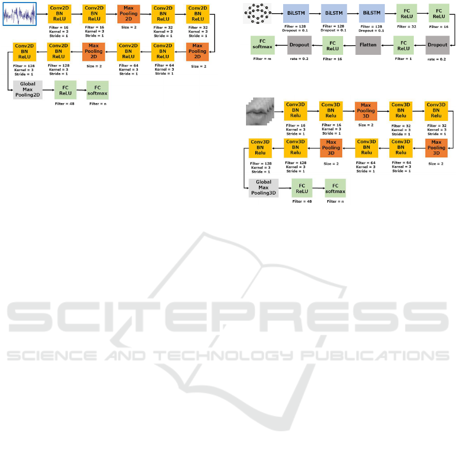
Figure 4: An overview of our ASR model.

n = the number of classes to conduct classiﬁcation.

5 ASR, VSR AND AVSR

In this section, we introduce our multi-angle AVSR

method based on late-fusion approach proposed in

(S.Isobe et al., 2021c), as well as ASR and VSR tech-

niques.

5.1 ASR

In our ASR framework, we extract mel-frequency

spectrograms that are commonly used for CNN-based

speech recognition. We then choose a 2D CNN model

illustrated in Fig. 4. The model employs a simple

and common architecture; convolutional and pool-

ing layers are repeatedly applied followed by Fully-

Connected (FC) layers, to get a classiﬁcation result.

In addition, by adding augmentation data in which

acoustic noise is added to original utterances, we can

compensate the lack of training data and make the

ASR model robust against acoustic noise.

5.2 Multi-angle VSR

We adopt a multi-angle VSR method consisting of

several angle-speciﬁc models as well as an angle esti-

mation, proposed in our previous work (S.Isobe et al.,

2021c). The conventional multi-angle VSR research

works have angle-speciﬁc VSR models. However,

these methods do not take into account the problem:

at which angle the lip image will be input. We de-

signed our multi-angle VSR so that the model could

properly deal with any angle lip images by involving

an angle classiﬁer. Each angle-speciﬁc VSR model is

trained using not only lip images at the correspond-

ing angle, but also those at the surrounding two an-

gles. For instance, a VSR model for 45

◦

is build

from 30

◦

, 45

◦

and 60

◦

lip data. We have already

conﬁrmed in previous research works that this can

achieve higher recognition accuracy than a conven-

tional scheme training a model with lip images at one

single angle only.

Figure 5: An overview of angle-speciﬁc VSR model.

n = the number of classes to conduct classiﬁcation.

Figure 6: An overview of angle estimation model.

m = the number of the angles.

5.2.1 Angle Estimator

The angle estimation module estimates conditional

probabilities for several angles, employing a Bi-

LSTM architecture. The module is illustrated in Fig.

5. The input is a sequence of lip feature points

which are obtained using face-alignment (A.Bulat and

G.Tzimiropoulos, 2017). As mentioned in detail later,

in this article we use two corpora. We choose the

following ﬁve angles for OuluVS2: 0

◦

(frontal), 30

◦

, 60

◦

and 90

◦

(proﬁle). For GAMVA, the follow-

ing 12 angles are chosen: 0

◦

(frontal), 0

◦

upper, 0

◦

lower, 10

◦

, 20

◦

, 30

◦

, 40

◦

, 50

◦

, 60

◦

, 70

◦

, 80

◦

and 90

◦

(proﬁle). Hence, the output layer consists of ﬁve units

for OuluVS2 or twelve units for GAMVA, each cor-

responding to one of the above angles.

5.2.2 Angle-speciﬁc VSR

We put several angle-speciﬁc VSR models in our

framework. The framework of each VSR model is

shown in Fig. 6. One VSR model is trained on not

only with lip images at the corresponding angle, but

also with those at neighboring two angles, having a

3D CNN architecture. Since the task when using

OuluVS2 in this paper is a 10-class classiﬁcation, the

last FC layer has 10 units, each corresponding to a

class probability. For GAMVA, because the task is a

25-class classiﬁcation, the last layer has 25 units.

5.3 AVSR

Firstly, a sequence of lip feature points is accepted

to the angle estimator model. Second, a sequence

ICPRAM 2022 - 11th International Conference on Pattern Recognition Applications and Methods

454

Table 1: Data Speciﬁcation of OuluVS2.

Noise #spkr #data

Train

Audio

Clean 35 1,050

#Random 35 1,050

Visual Clean (/angle) 35 1,050

Valid

Audio

Clean 5 150

#Random 5 150

Visual Clean (/angle) 5 150

Test

Audio

Clean 12 360

Park (/SNR) 12 360

Metro (/SNR) 12 360

Visual Clean (/angle) 12 360

#spkr = the number of the subjects.

#data = the number of the utterance data.

Table 2: Data Speciﬁcation of GAMVA.

Noise #spkr #data

Train

Audio

Clean 12 900

#Random 12 900

Visual Clean (/angle) 12 900

Valid

Audio

Clean 3 225

#Random 3 225

Visual Clean (/angle) 3 225

Test

Audio

Clean 5 375

Park (/SNR) 5 375

Metro (/SNR) 5 375

Visual Clean (/angle) 5 375

of lip images is submitted to all VSR models, while

corresponding speech data are recognized in the ASR

model.

As mentioned, the tasks of OuluVS2 and GAMVA

are 10-class and 25-class classiﬁcation respectively.

We obtain results from ASR and VSR modules as

conditional probabilities for every classes. Let us de-

note a probability for an i-th class from a j-th angle-

speciﬁc model by V

i, j

, with w

that is a conditional

probability for a j-th angle estimation model, and a

score from ASR by A

. Angle-speciﬁc recognition

results are integrated by the angle estimation scores

to make the VSR result based on the decision-fusion

manner, and with audio classiﬁcation result, ﬁnally

the class having the highest score is selected as:

i = argmax

∑

j=1

i, j

, (8)

where m is the number of angles.

6 EXPERIMENT

6.1 Database

In this research, we selected two multi-angle audio-

visual corpora: OuluVS2 and GAMVA. DEMAND

Table 3: Utterances in GAMVA.

Japanese pronunciation English meaning

/a-ri-ga-to-u/ thank you

/i-i-e/ no

/o-ha-yo-u/ good morning

/o-me-de-to-u/ congratulation

/o-ya-su-mi/ good night

/go-me-N-na-sa-i/ I’m sorry

/ko-N-ni-chi-wa/ good afternoon

/ko-N-ba-N-wa/ good evening

/sa-yo-u-na-ra/ good bye

/su-mi-ma-se-N/ excuse me

/do-u-i-ta-shi-ma-shi-te/ you are welcome

/ha-i/ yes

/ha-ji-me-ma-shi-te/ nice to meet you

/ma-ta-ne/ see you

/mo-shi-mo-shi/ hello

/ba-i-ba-i/ bye bye

/i-ta-da-ki-ma-su/ I’ll take it

/go-chi-so-u-sa-ma/ thank you for meal

/o-tsu-ka-re-sa-ma/ see you

/ta-da-i-ma/ I’m home

/o-ka-e-ri/ welcome home

/o-jya-ma-shi-ma-su/ excuse me for disturbing you

/si-tsu-re-i-shi-ma-su/ excuse me

/hi-sa-shi-bu-ri/ long time no see

/yo-ro-shi-ku/ nice to meet you

database was also used as a noise corpus.

6.1.1 OuluVS2

We chose the OuluVS2 corpus (I.Anina et al., 2015)

to evaluate our scheme. The database contains 10

short phrases, 10 digits sequences, and 10 TIMIT sen-

tences uttered by 52 speakers. The corpus includes

face images captured by ﬁve cameras simultaneously

at 0

◦

(frontal), 30

◦

, 45

◦

, 60

◦

, and 90

◦

(proﬁle) angles,

respectively. In this paper, we adopted the phrase

data, uttered three times by each speaker. In our ex-

periment, the data spoken by 52 speakers were di-

vided into training data by 35 speakers, validation

data by 5 speakers and testing data by 12 speakers.

We also checked whether the data split was appropri-

ate by changing the different split settings, and con-

ﬁrmed that using the data sets could give us the fair

results. The phrases are as follows: ”Excuse me”,

”Goodbye”, ”Hello”, ”How are you”, ”Nice to meet

you”, ”See you”, ”I am sorry”, ”Thank you”, ”Have a

good time”, ”You are welcome”.

6.1.2 GAMVA

We also used the GAMVA corpus (S.Isobe et al.,

2021a), which was build in our previous work. The

database contains Japanese greeting phrases shown

in Table 3 spoken by 20 male subjects. The corpus

Efﬁcient Multi-angle Audio-visual Speech Recognition using Parallel WaveGAN based Scene Classiﬁer

455

includes face movies simultaneously captured by 12

cameras: 0

◦

(frontal), 0

◦

upper, 0

◦

lower, 10

◦

, 20

◦

, 40

◦

, 50

◦

, 60

◦

, 70

◦

, 80

◦

and 90

◦

(proﬁle). Among

them, 10 movies can be used to evaluate horizontal

difference, while 3 movies are for vertical difference:

◦

, 0

◦

upper and 0

◦

lower. Face feature points and

speech sounds are also involved in this corpus. Each

subject uttered the same contents three times, similar

to OuluVS2. In our experiment, the data spoken by 20

speakers were divided into training data by 12 speak-

ers, validation data by 3 speakers and testing data by

5 speakers.

6.1.3 DEMAND

We selected another database DEMAND (J.Thiemann

et al., 2013) as a noise corpus. This corpus consists of

six primary categories, each which has three environ-

ments, respectively. Four of those primary categories

are for closed spaces: Domestic, Ofﬁce, Public, and

Transportation. And the remaining two categories are

recorded outdoors: Nature and Street. In this paper,

we added some kinds of those noises to build audio

training and testing data.

6.2 Experimental Setup

We evaluated a model by utterance-level accuracy:

Accuracy =

× 100 [%] (9)

where H and S are the number of correctly recog-

nized utterances and the total number of utterances,

respectively. Since DNN-based model performance

slightly varies depending on the probabilistic gradi-

ent descend algorithm, that is a common model train-

ing approach, we repeated the same experiment ﬁve

times and the mean accuracy was calculated. In terms

of DNN hyperparameters of speech recognition, we

chose a cross-entropy function as a loss function.

Adam was used for all DNNs as an optimizer. Batch

size, epochs and learning rate were set to 32, 50 and

0.001, respectively. Regarding of training of Paral-

lel WaveGAN, we set batch size, epochs and learn-

ing rate as 10, 1000 and 0.0001, respectively. We

carried out our experiments using NVIDIA GeForce

RTX 2080 Ti.

6.3 Preprocessing

6.3.1 Utterance

In the OuluVS2 data set, there are 1,050 (35 speak-

ers × 10 utterance × 3times) sentences available for

training, 150 (5 speakers × 10 utterance × 3times)

sentences available for validation and 360 (12 speak-

ers × 10 utterance × 3times) sentences for testing.

However, the data size is not enough for DNN model

training. To compensate the lack of training data,

we applied data augmentation in the audio and vi-

sual modalities. In the audio modality, we added

three types of acoustic noises in DEMAND to orig-

inal training utterance data. At this time, noise type

and Signal-to-Noise Ratio (SNR) were randomly de-

termined. In addition, we added different types of

acoustic noises to testing data. The details including

noise kind and SNR conditions are shown in Table 1.

In the visual modality, we trained our VSR models

using not only lip images at one angle, but also those

at the neighbor two angles.

In the GAMVA data set, there are 900 (12 speak-

ers × 25 utterance × 3times) sentences for training,

225 (3 speakers × 25 utterance × 3times) sentences

available for validation and 375 (5 speakers × 25 ut-

terance × 3times) sentences for testing. The same

data augmentation was conducted. Details including

noise kind SNR conditions are shown in Table 2.

6.3.2 Audio and Image Processing

The OuluVS2 data set includes face movies (1920 ×

1080) and audio speech data. In the visual modality,

as described in Section 4, we ﬁrstly converted face

movies to face image sequences. Next, we detected

68 face feature points on each image, followed by ex-

tracting a lip image. Because cropped lip images had

different sizes, we resized all images to 128×128 in

order to apply DNNs. Furthermore, we normalized

a frame length to 24; if the sequence length was less

than 24 we conducted upsampling, otherwise we sup-

pressed some frames. In addition, we converted all

color images to gray-scale ones. Similar to visual

frames, we normalized an audio frame length to 32

by resizing the mel-frequency spectrogram in the time

direction.

GAMVA data set has face movies (1280 × 720)

and audio speech data. We conducted the similar pre-

processing as OuluVS2. We set the image size, the

image frame length and the audio frame length as

64×64, 48, 72, respectively.

6.4 Results and Discussion

6.4.1 Scene Classiﬁcation

The result of scene classiﬁcation is shown in Table

4. At ﬁrst, we discuss the result of OuluVS2. In

the case of SNR 0dB and 5dB, where the effect of

acoustic noise were large, most of the data could be

correctly classiﬁed as noisy. However, in the case

ICPRAM 2022 - 11th International Conference on Pattern Recognition Applications and Methods

456

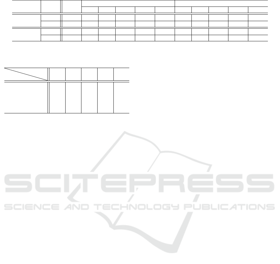
Table 4: Scene classiﬁcation results.

corpus env clean

Park Metro

0dB 5dB 10dB 15dB 20dB 0dB 5dB 10dB 15dB 20dB

OuluVS2

clean 243 5 55 147 213 239 2 40 140 221 247

noisy 116 354 304 212 146 120 357 319 219 138 112

GAMVA

clean 372 0 0 62 269 352 0 59 287 367 371

noisy 0 372 372 310 103 20 372 313 85 5 1

Table 5: A Confusion Matrix in View Classiﬁcation for

OuluVS2.

Result

Label

◦

360 0 0 0 0

◦

0 340 39 2 0

◦

0 20 148 42 0

◦

0 0 173 315 0

◦

0 0 0 0 198

of SNR 15dB, 20dB and clean environment, where

the effect of noise were small, misclassiﬁcation often

occurred. Regarding GAMVA, on the contrary, we

could achieve signiﬁcantly higher accuracy among all

SNR conditions. In particular, in the case of SNR 0dB

and clean, the estimator classiﬁed all the testing data

completely.

Assume that given noisy data are misclassiﬁed as

clean. Only speech recognition is then conducted, re-

sulting that the recognition accuracy is reduced. On

the contrary, when input clean data are miscategorized

into the noisy speech, the multi-angle AVSR is con-

ducted; the processing time becomes then longer than

ASR only, but the recognition accuracy is expected

to be still high. Focusing on the results of OuluVS2,

the scene classiﬁer sometimes judged noisy data as

clean. Such the misclassiﬁcation was not severe in

terms of speech recognition, because AVSR was car-

ried out instead of ASR, but the reduction of computa-

tional cost was no longer expected. We checked gen-

erated utterances by Parallel WaveGAN, and found

that the generator model was able to generate not only

utterances but also background noise in OuluVS2. On

the other hand, in the case of GAMVA, the generator

only regenerated utterances. This might cause such

the differences in terms of scene classiﬁcation results.

The reason why the generator reconstructed noise in

OuluVS2 should be further investigated, but we con-

sider utterance speed and phonetic differences might

affect the performance.

6.4.2 View Classiﬁcation

Here we investigated view classiﬁcation performance.

Table 5 and Table 6 show view classiﬁcation con-

fusion matrices. The classiﬁcation accuracy for

OuluVS2 is 83.14%, and the accuracy for GAMVA

is 57.96%. As described already, each angle-speciﬁc

VSR model was trained using lip images at three an-

gles. Taking this into account, we may evaluate the

models by counting not only correctly classiﬁed ut-

terances but also utterances classiﬁed into the next

angle. In the case, the accuracy for OuluVS2 rises

to 99.88%, and the accuracy for GAMVA becomes

95.78%. It is consequently conﬁrmed that our angle

estimation model was able to estimate the angle of the

input lip images, without affecting the performance of

following lip-reading modules.

6.4.3 Speech Recognition

Subsequently, we discuss speech recognition results.

Table 7 and Table 8 show recognition accuracy

of our ASR, VSR, AVSR and our proposed scene

classiﬁcation-based recognition methods under two

testing noise environments for two multi-angle audio-

visual data sets, OuluVS2 and GAMVA, respectively.

Note that, because the task was a 10-class or a 25-

class classiﬁcation respectively, the accuracy in noisy

environments tended to be higher compared to large-

vocabulary speech recognition.

First, we discuss the results of the ASR method.

Since audio waveforms were polluted by acoustic

noise, the lower the SNR was, the lower recognition

accuracy became. Based on the recognition results

and the scene classiﬁcation results, it turns out that

15dB or higher can be considered as ”clean” environ-

ments; the recognition accuracy of 15dB and 20dB

was almost equivalent to that in the clean environ-

ments.

Second, we focus on the results of the multi-angle

VSR method. Table 9 and Table 10 show the recog-

nition accuracy of each angle, in addition to the mean

accuracy among all the angles with or without angle

estimation in the data sets, respectively. The VSR

accuracy was stable and unrelated to SNR since vi-

sual information is not basically affected by acous-

tic noise. Note that, the VSR result of Table 7 and

Table 8 corresponds to the mean accuracy in Table

9 and Table 10 with the angle estimator. As widely

known, the results of VSR were not better than those

of ASR in all the SNRs, because audio features are

Efﬁcient Multi-angle Audio-visual Speech Recognition using Parallel WaveGAN based Scene Classiﬁer

457

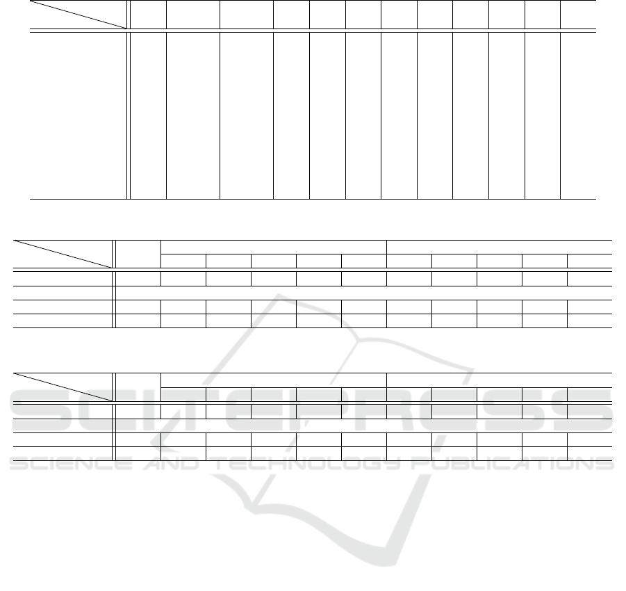
Table 6: A Confusion Matrix in View Classiﬁcation for GAMVA.

Result

Label

◦

(lower) (upper)

◦

130 154 31 11 0 0 0 0 0 0 0 0

◦

(lower) 56 71 19 2 0 0 0 0 0 0 0 0

◦

(upper) 99 107 136 3 0 0 0 0 0 0 0 0

◦

90 43 189 301 5 0 0 0 0 0 0 0

◦

0 0 0 58 288 11 0 0 0 0 0 0

◦

0 0 0 0 82 322 51 0 0 0 0 0

◦

0 0 0 0 0 42 259 93 1 0 0 0

◦

0 0 0 0 0 0 65 216 75 1 0 0

◦

0 0 0 0 0 0 0 66 295 159 11 0

◦

0 0 0 0 0 0 0 0 4 210 145 29

◦

0 0 0 0 0 0 0 0 0 5 205 171

◦

0 0 0 0 0 0 0 0 0 0 14 175

Table 7: ASR, VSR and AVSR Accuracy [%] in Various Noise Conditions in OuluVS2.

Model

Data

clean

Park Metro

0dB 5dB 10dB 15dB 20dB 0dB 5dB 10dB 15dB 20dB

ASR 95.83 93.17 95.56 95.78 95.89 95.94 92.33 95.94 95.78 95.83 95.83

VSR 83.00

AVSR 97.88 96.53 97.61 97.88 97.99 97.92 96.42 97.69 97.80 97.81 97.84

AVSR with SC 96.84 96.34 97.20 96.82 96.76 96.73 96.42 97.44 96.92 96.53 96.64

Table 8: ASR, VSR and AVSR Accuracy [%] in Various Noise Conditions in GAMVA.

Model

Data

clean

Park Metro

0dB 5dB 10dB 15dB 20dB 0dB 5dB 10dB 15dB 20dB

ASR 94.35 92.69 93.87 94.19 94.40 94.40 90.19 92.91 94.03 94.19 94.29

VSR 78.47

AVSR 97.78 96.72 97.52 97.72 97.76 97.76 95.70 96.88 97.43 97.60 97.73

AVSR with SC 94.35 96.72 97.52 97.53 96.43 94.86 95.70 96.53 96.01 94.49 94.29

generally more effective and informative than visual

cues. It is found that the recognition accuracy of 90

◦

in OuluVS2 was about 5-8% lower than the other an-

gles. This is due to the fact that, the face alignment

used to crop lip images sometimes failed to detect fa-

cial landmarks, which might be caused by less train-

ing data. In other words, this is not because of the an-

gle, but because of the small number of training data

for face alignment.

Third, we discuss the results of the multi-angle

AVSR method. Among the models, AVSR achieved

the best accuracy in all the conditions. As mentioned,

we employed the decision-fusion strategy, which is

the simplest integration method, because the recog-

nition task in this paper was a kind of classiﬁcation.

Similar to an ensemble approach, we consider our

decision-fusion method could successfully integrate

ASR and VSR results, which had different recogni-

tion errors.

Finally, we discuss the results of our pro-

posed multi-angle AVSR with the scene classiﬁcation

method. When SNR was 10dB or lower which was

regarded as noisy environments, the recognition ac-

curacy was almost the same as AVSR, and was still

improved compared to the accuracy of ASR. As al-

ready denoted, in the lower SNR environments AVSR

was usually selected, as a result, we could keep the

accuracy. On the other hand, when SNR was 15dB or

higher which was regarded as clean environments, the

recognition accuracy was lower than AVSR, but was

slightly higher than ASR.

6.4.4 Processing Time

Here we focus on processing time of ASR, multi-

angle AVSR and our proposed multi-angle AVSR us-

ing scene classiﬁcation. Table 11 shows the process-

ing time of each speech recognition in the two data

sets.

At ﬁrst, we focus on the results of the OuluVS2.

The processing time of inference of ASR model was

205 sec. The processing time was measured during

recognizing not only clean data but also ﬁve-level

SNR data of the two types of noise in the test set; the

total number of utterances was thus 3,960 (= 360 ×

11), and the length of utterances was 2,552 (= 232 ×

ICPRAM 2022 - 11th International Conference on Pattern Recognition Applications and Methods

458

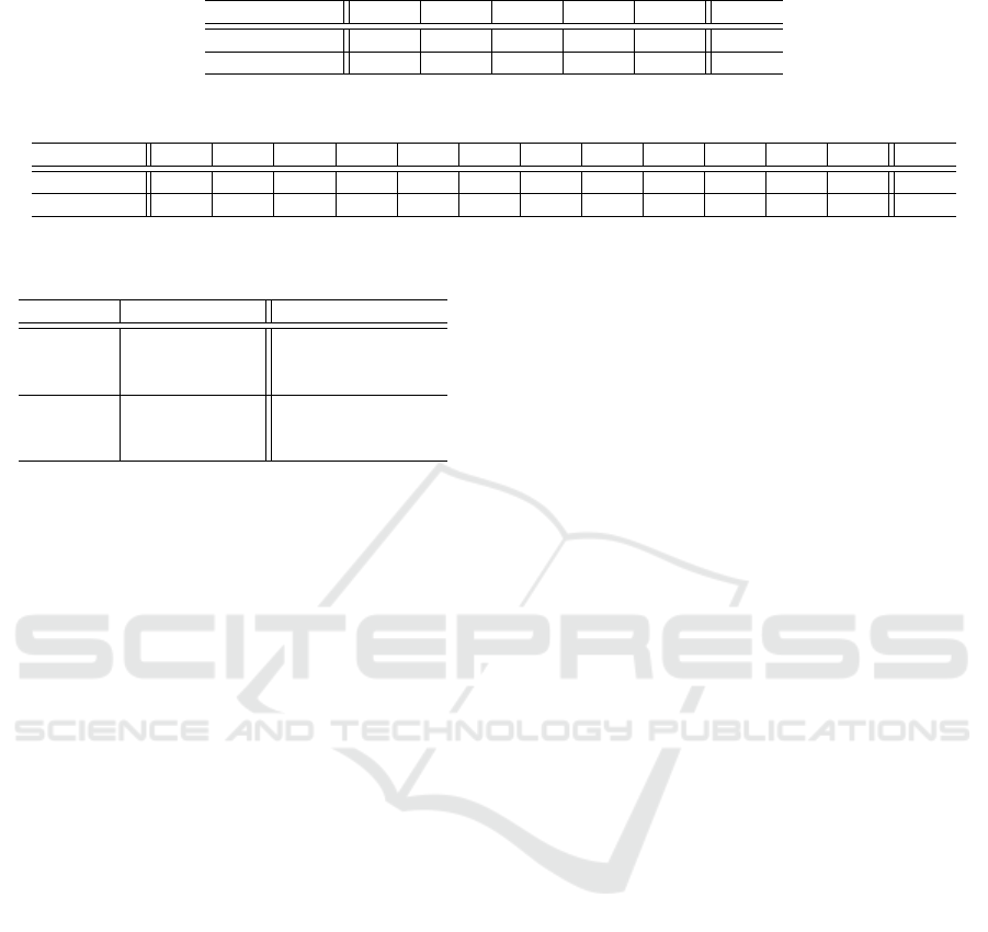
Table 9: Recognition accuracy (%) of multi-angle VSR with or without angle estimation in OuluVS2 data set.

◦

Mean

Without AEM 85.39 85.28 84.44 83.30 77.47 83.18

With AEM 85.39 85.11 84.50 82.51 77.47 83.00

AEM = Angle Estimation Module.

Table 10: Recognition accuracy (%) of multi-angle VSR with or without angle estimation in GAMVA data set.

◦

(l) 0

◦

(u) 10

◦

Mean

Without AEM 77.97 76.96 78.08 81.60 77.87 81.12 79.31 76.64 75.09 74.67 70.08 68.75 76.38

With AEM 84.48 79.52 80.05 82.35 79.36 82.67 80.37 77.65 75.95 75.31 74.67 69.28 78.47

AEM = Angle Estimation Module, 0

◦

(l) = 0

◦

from the lower camera, 0

◦

(u) = 0

◦

from the upper camera.

Table 11: Processing time.

corpus Model processing time (s)

OuluVS2

ASR 205

AVSR 24,553

AVSR with SC 16,586

GAMVA

ASR 112

AVSR 27,872

AVSR with SC 18,605

11) sec. Second, the processing time of multi-angle

AVSR was 24,553 sec. The most of the processing

time was for detection of face landmark using face

alignment, and extraction of lip images using detected

facial landmark. On the other hand, the processing

time of multi-angle AVSR using our scene classiﬁca-

tion was 16,586 sec. Our proposed method was able

to reduce processing time compared to the conven-

tional multi-angle AVSR method. In GAMVA data

set, we found the same result as OuluVS2 data set.

7 CONCLUSION

In this paper, we proposed a scene classiﬁcation based

multi-angle AVSR method to reduce processing time

of AVSR keeping the recognition accuracy as much

as possible. The scene classiﬁer predicted a record-

ing condition; given speech data were recorded ei-

ther clean or noisy environments. Only ASR was ap-

plied to the clean data, whereas AVSR with multi-

angle VSR was carried out for noisy speech data.

We conducted experiments to evaluate effectiveness

and efﬁciency of our proposed method, using two

multi-angle AVSR data set: OuluVS2 and GAMVA.

Then we found that our scheme could conduct ro-

bust speech recognition against acoustic noise than

the ASR method, and reduce processing time than

the multi-angle AVSR method. As our future work,

we are planning to conduct our proposed method for

large-vocabulary speech recognition. In addition, cur-

rently, many neural vocoder methods other than Par-

allel WaveGAN have been proposed. In this paper,

we used Parallel WaveGAN, but we are planning to

examine the results of scene classiﬁcation when other

methods are used.

REFERENCES

A.Bulat and G.Tzimiropoulos (2017). How far are we from

solving the 2D & 3D Face Alignment problem? (and

a dataset of 230,000 3D facial landmarks). In arXiv

preprint arXiv:1703.07332.

A.Koumparoulis and G.Potamianos (2018). Deep

view2view mapping for view-invariant lipreading. In

Proc. SLT, pp.588–594.

A.Oord, S.Dieleman, H.Zen, K.Simonyan, O.Vinyals,

A.Graves, N.Kalchbrenner, A.Senior, and

K.Kavukcuoglu (2016). WaveNet: A genera-

tive model for raw audio. In arXiv preprint

arXiv:1609.03499.

G.Paraskevopoulos, S.Parthasarathy, A.Khare, and

S.Sundaram (2020). Multiresolution and Multimodal

Speech Recognition with Transformers. In arXiv

preprint arXiv:2004.14840v1.

I.Anina, Z.Zhou, G.Zhao, and Pietik

aine, M. (2015).

OuluVS2: A multi-view audiovisual database for non-

rigid mouth motion analysis. In Proc. 11th IEEE In-

ternational Conference and Workshops on Automatic

Face and Gesture Recognition (FG).

J.Kong, J.Kim, and J.Bae (2020). HiFi-GAN: Generative

Adversarial Networks for Efﬁcient and High Fidelity

Speech Synthesis. In In Advances in Neural Informa-

tion Processing Systems.

J.Thiemann, N.Ito, and E.Vincent (2013). DEMAND: a col-

lection of multichannel recordings of acoustic noise in

diverse environments. In Proc. ICA.

K.Inagaki, S.Tamura, and S.Hayamizu (2020). Using Deep-

Learning Approach to Detect Anomalous Vibrations

of Press Working Machine. In Sensors and Instru-

mentation, Aircraft/Aerospace, Energy Harvesting &

Dynamic Environments Testing, Volume 7. Springer.

K.Kumar, R.Kumar, Boissiere, T., L.Gestin, W.Z.Teoh,

J.Sotelo, Brebisson, A., Y.Bengio, and A.Courville

(2019). MelGAN: Generative Adversarial Networks

for Conditional Waveform Synthesis. In In Advances

in Neural Information Processing Systems.

K.Suefusa, T.Nishida, H.Purohit, R.Tanabe, T.Endo, and

Y.Kawaguchi (2020). Anomalous Sound Detection

Efﬁcient Multi-angle Audio-visual Speech Recognition using Parallel WaveGAN based Scene Classiﬁer

459

Based On Interpolation Deep Neural Network. In

Proc. ICASSP, pp. 271-275.

P.Zhou, W.Yang, W.Chen, Y.Wang, and J.Jia (2019).

Modality attention for end-to-end audio-visual speech

recognition. In arXiv preprint arXiv:1811.05250v2.

R.Yamamoto, E.Song, and J.-M.Kim (2020). Paral-

lel WaveGAN: A fast waveform generation model

based on generative adversarial networks with multi-

resolution spectrogram. In Proc. ICASSP, pp.

6199–6203.

S.Isobe, R.Hirose, T.Nishiwaki, T.Hattori, S.Tamura,

Y.Gotoh, and M.Nose (2021a). GAMVA: A Japanese

Audio-Visual Multi-angle Speech Corpus. In Proc.

Oriental COCOSDA.

S.Isobe, S.Tamura, and S.Hayamizu (2021b). Speech

Recognition using Deep Canonical Correlation Anal-

ysis in Noisy Environments. In PRoc. ICPRAM, pp.

63-70.

S.Isobe, S.Tamura, S.Hayamizu, Y.Gotoh, and M.Nose

(2020). Multi-angle lipreading using angle classiﬁ-

cation and angle-speciﬁc feature integration. In Proc.

ICCSPA. IEEE.

S.Isobe, S.Tamura, S.Hayamizu, Y.Gotoh, and M.Nose

(2021c). Multi-angle Audio-Visual Speech Recogni-

tion. In Proc. NCSP, pp. 369-372.

S.Isobe, S.Tamura, S.Hayamizu, Y.Gotoh, and M.Nose

(2021d). Multi-Angle Lipreading with Angle

Classiﬁcation-Based Feature Extraction and Its Appli-

cation to Audio-Visual Speech Recognition. In Future

Internet, Vol.13, Issue.7. MDPI.

S.Petridis, T.Stafylakis, P.Ma, F.Cai, G.Tzimiropoulos, and

M.Pantic (2018). End-to-end multiview lip reading.

In Proc. ICASSP, pp.6548–6552.

S.Petridis, Y.Wang, Z.Li, and M.Pantic (2017). End-to-End

Audiovisual Fusion with LSTMs. In Proc. AVSP.

T.Makino, H.Liao, Y.Assael, B.Shillingford, B.Garcia,

O.Braga, and O.Siohan (2019). Recurrent neural net-

work transducer for audio-visual speech recognition.

In arXiv preprint arXiv:1911.04890v1.

X.Mao, Q.Li, H.Xie, Lau, R., Z.Wang, and S.P.Smolley

(2017). Least Squares Generative Adversarial Net-

works. In Proc. ICCV, pp. 2794-2802.

Y.Koizumi, Y.Kawaguchi, K.Imoto, T.Nakamura,

Y.Nikaido, R.Tanabe, H.Purohit, K.Suefusa, T.Endo,

M.Yasuda, and N.Harada (2020). Description and

Discussion on DCASE2020 Challenge Task2: Unsu-

pervised Anomalous Sound Detection for Machine

Condition Monitoring. In DCASE2020 Workshop /

arXiv preprint arXiv:2006.05822.

ICPRAM 2022 - 11th International Conference on Pattern Recognition Applications and Methods

460