
Multi-view NURBS Volume
Wanwan Li
Department of Computer Science
George Mason University, Fairfax, VA, U.S.A.
Keywords:
Geometric Modeling, Interactive Interface, Numerical Optimization, NURBS Volume.
Abstract:
Non-Uniform Rational B-Spline (NURBS) curves and surfaces are widely used in modern geometric model-
ing systems. NURBS volumes, also called volumetric NURBS, are one powerful NURBS representation of
volumetric modeling. However, due to the complex nature of NURBS volumes, it is a challenging task for
users to fine-tune the NURBS volumes design manually. In this paper, we present a novel approach for multi-
view NURBS volume geometric modeling. Given users’ conceptual design for several different views of a
3D model, we devise an optimization algorithm to automatically reconstruct the 3D NURBS volume which is
matching with these designs by projecting it along with different view directions. In the end, we discuss the
results generated with our approach through a series of numerical experiments.
1 INTRODUCTION
Non-Uniform Rational B-Spline (NURBS) is a math-
ematical formulation that represents the controllable
geometry of curves and surfaces in 2D or 3D space.
NURBS curves and surfaces can be precisely created
and edited by users through control points. There-
fore, modern 3D modeling software such as Autodesk
3Ds Max, Maya, Blender, SketchUp, Revit, Rhino,
Camera 4D, etc. all support the input as NURBS ge-
ometry. Due to the controllability of NURBS curves
and surfaces, they are widely used in digital art de-
sign, industrial design, architectural design, game de-
sign, and animation movie industry, etc. There are
a great number of researches on user interface stud-
ies for computer-aided designs (CAD) that are mostly
focused on the NURBS curves and surfaces for devel-
oping smarter interfaces of 2D or 3D modelings.
However, as another natural extension of NURBS
curves and surfaces, NURBS volumes design is an-
other interesting topic to explore. NURBS volumes
are scalar fields who are consisting of a couple of
scalar numbers. Those scalar numbers are controlled
by some control values. Volumetric data are com-
mon in the data processing and data visualization
community. Especially, volumetric data are often
used in medical science, boolean operations, and
points clouds computing, etc. Therefore, volumet-
ric NURBS have great potential to be connected with
volumetric data processing and volumetric 3D mod-
eling directly. Unfortunately, due to the complexity
of controlling the NURBS volumes and large com-
putation complexity, the application of volumetric
NURBS has not been widely studied so far and it still
remains an open challenge to design a smart interface
for controllable NURBS volume design. Given these
observations, we devise the first user controllable in-
terface for smart volumetric NURBS design. Through
our approach presented in this paper, users can design
their expected NURBS volumes through digital de-
signs on three different views, front view, left view,
and top view. As shown in Figure 1 (a), given these
input from an arbitrary device (in this case, a cell
phone), we visualize them onto three orthogonal walls
in Unity3D (b); and optimize the NURBS volume so
that it can automatically match with three-views after
being projected along three-axis (c). The main contri-
butions of our work include:
• Opening an interesting topic about design-driven
multi-view NURBS volume modeling.
• Devising an optimization approach to automati-
cally fine-tune the NURBS volumes to match with
users’ input of designs on different views.
• Conducting a series of numerical experiments to
validate our approach and discuss its limitations.
2 RELATED WORK
NURBS Geometry Reconstruction. Using NURBS-
based geometry to reconstruct objects’ 2D profile
curves or 3D manifold surfaces is a popular re-
search topic. Since the late 20th century, (Lavoie
et al., 1999), camera views-based NURBS shapes
228
Li, W.
Multi-view NURBS Volume.
DOI: 10.5220/0010850200003124
In Proceedings of the 17th International Joint Conference on Computer Vision, Imaging and Computer Graphics Theory and Applications (VISIGRAPP 2022) - Volume 1: GRAPP, pages
228-235
ISBN: 978-989-758-555-5; ISSN: 2184-4321
Copyright
c
2022 by SCITEPRESS – Science and Technology Publications, Lda. All rights reserved
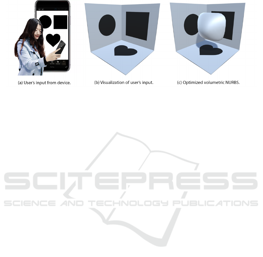
Figure 1: Demo of multi-view volumetric NURBS design. (a) Given the user’s digital painting of shapes projected from three
view directions including the front, top, and left view, (b) The User’s three-view design is visualized on three walls in the
Unity3D interface. (c) Finally, we optimize the NURBS volume to match with such a design from the three view directions.
modeling has been widely studied. For example,
a high-precision technique for reconstructing three-
dimensional (3D) objects from its one-camera 2D
views and using a color-coded structured light is de-
scribed by Lavoie et al. (Lavoie et al., 1999). In their
approach, the lines extracted from a view of the ob-
ject are used for constructing the NURBS curves so
as to generate the surface of the object. In 2008, Pal
et al. (Pal, 2008) proposed a reconstruction method
using geometric subdivision and NURBS interpola-
tion to successfully bridge the geometric subdivi-
sion and NURBS reconstruction on subdivided data,
NURBS patch and topology planning, construction
of trimmed NURBS surfaces, and writing IGES of
result patches. At the same time, the NURBS ge-
ometry model has been applied in digital terrain re-
construction for hydropower engineering based on
the TIN model proposed by Zhong et al. (Zhong
et al., 2008). In 2012, Imani et al. (Imani and
Hashemian, 2012) reconstructed the 2D profiles us-
ing a constrained local fitting algorithm to approx-
imate the points segments through NURBS curves
with geometric continuity conditions. Later, in 2018,
Hashemian et al. (Hashemian and Hosseini, 2018)
propose an integrated approach for fitting and fair-
ing smooth NURBS curves and surfaces simultane-
ously to reconstruct 3D objects elegantly through op-
timizations. At the same time, the article proposed
by (Vu-Bac et al., 2018) presents a gradient-based op-
timization algorithm to recover the applied loads and
deformations of thin shell structures through NURBS
geometry. NURBS curves can also be applied in tra-
jectory reconstruction for robot programming (Ale-
otti et al., 2005). Multi-view-based reconstruction
on NURBS curves has been successfully explored by
Saini et al. (Saini et al., 2015). In their project, two
perspective images defining the curves are used as the
input and a nonlinear optimization process is used to
fit a NURBS curve on the projected curves in these
images. Later, the same group (Saini et al., 2021)
proposed a two-view-based free-form NURBS curve
shape reconstruction algorithm using the Generalized
Ant Colony Optimizer (GACO) model. However,
none of the existing work has explored using NURBS
volumes to represent the 3D shapes of users’ geomet-
ric modelings and designs. Therefore, in this paper,
we explore the possibility and capability of interac-
tive controllable NURBS volume modeling.
Multi-view Geometric Modeling. Besides those
works on multi-view NURBS curves reconstructions
mentioned earlier, there are lots of other works
on multi-view geometric modeling. In computer
stereo vision, calibration images are mostly used for
3D shape reconstruction. For example, Sinha et
al. (Sinha and Pollefeys, 2005) describes a novel ap-
proach for reconstructing a closed continuous sur-
face from multiple calibrated color images and sil-
houettes by strictly enforces silhouette constraints
and optimize photo consistency with smoothness at
the same time. Labatut et al. (Labatut et al., 2007)
proposed approach focused on large-scale cluttered
scenes under uncontrolled imaging conditions. Later,
Fuhrmann et al. (Fuhrmann et al., 2014) proposed
MVE, an aulti-view reconstruction environment that
takes into consideration the structure-from-motion
(SfM) techniques, depth maps estimation using multi-
view stereo (MVS), and colored mesh extraction us-
ing a surface reconstruction approach called FSSR.
The work most closely related to our work is the
framework for multi-view wire art design proposed by
Hsiao et al. (Hsiao et al., 2018). In this work, an op-
timization approach is devised to optimize a wire art
design which can be projected along different view
directions to generate different sketchings that look
the same as the users’ inputs. This work inspires us
to devise an optimization algorithm to synthesize a
Multi-view NURBS Volume
229
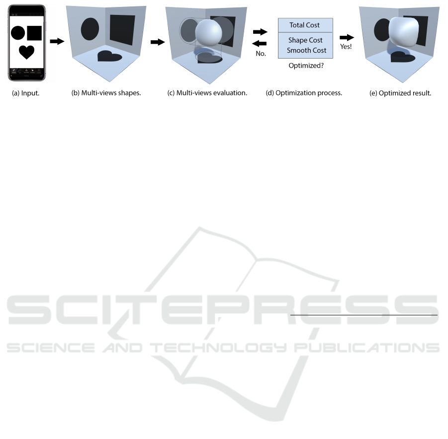
Figure 2: Overview ot our approach.
NURBS volume that can automatically match with
users’ inputs in a similar way.
3 OVERVIEW
Figure 2 shows the overview of our approach. (a)
Given the user’s input as the shapes defined from
three views, in this case, the user paints three dif-
ferent shapes through an app on a mobile device.
(b) we convert the shape images to binary images
and project them onto three different walls within a
3D scene modeled in Unity3D. (c) We initialize the
NURBS volume with control values of zeros and con-
trol weights of ones. We extract the NURBS isosur-
face with an isovalue of 0.5. Then, we evaluate the
correctness of the NURBS volume shape by project-
ing it onto three different views and compare them
with the user’s input shapes respectively, projected
shadows plotted as gray circle areas. (d) During the
optimization process, we consider two important as-
pects of the NURBS volume shape, the first is shape
cost which measures the difference between the gen-
erated NURBS volume and the user’s input according
to the evaluation process shown in (c). The second
is the smoothness of the generated NURBS volume,
as we hope it can be as smooth as possible. Without
this regularization term of smoothness cost, the re-
sulted NURBS volume will become rough and wrin-
kled so that the generated surface is not acceptable.
We will compare and discuss the effects of generated
NURBS isosurface with and without smooth costs
in the later section. For each optimization step, we
check whether the generated NURBS volume is op-
timized according to two considerations: (1) whether
the maximum number of iteration is reached and (2)
whether the total cost value is not changing which
means a local minimum is reached. If the result is
not optimized, we update the control values and con-
trol weights of the NURBS volume and go back to the
evaluation step shown in (c); Otherwise, we output the
final optimized result as shown in (e). As we can see
from the result shown in this example, the generated
NURBS volume has a shape that looks like the user’s
input where the front is a square, the left is a circle and
the top is a heart. The result isosurface of optimized
NURBS volume is a smooth manifold surface.
4 PROBLEM FORMULATION
NURBS Volume. We formulate the NURBS volume
as a continuous scalar field defined through m × n × l
control values V
i, j,k
and control weights W
i, j,k
, where
i ∈ [1,m], j ∈ [1,n], and k ∈ [1,l]. Then the scalar
field f (u,v, w) of NURBS volume at arbitrary position
(u,v,w) ∈ R
3
in the parameter space is calculated as:
f (u,v,w) =
∑
m
i
∑
n
j
∑
l
k
V
i, j,k
B
i
p
(u)B
j
q
(v)B
k
r
(w)W
i, j,k
∑
m
i
∑
n
j
∑
l
k
B
i
p
(u)B
j
q
(v)B
k
r
(w)W
i, j,k
,
where u,v, w ∈ [0,1] and B
i
p
(u), B
j
q
(v), B
k
r
(w) are p,
q, r-order B-spline base function at i, j, k-th control
values respectively. For simplicity, in this paper, we
use the same order for p, q, r as the control order o
for the NURBS volume. By default, we set o = 3.
NURBS Isosurface. We extract the isosurface of
NURBS volume given an arbitrary isovalue C such
that f (u,v,w) = C using a matching cube algorithm.
The isosurface is the result manifold surface that rep-
resents the NURBS volume. By default, we set the
isovalue C = 0.5. In the later section, we will change
the isovalue to discuss the differences in the synthe-
sized results. Our goal of the problem formulation is
to find an isosurface such that it can match with the
user’s input from different views as much as possible.
Total Cost Function. We formulate this problem as
an optimization problem to find the NURBS volume
scalar field function f
∗
(u,v,w) calculated by control
values V
∗
and control weights W
∗
that can minimize
the total cost function C
total
( f ) which is defined as:
C
total
( f ) = w
shape
C
shape
( f ) + w
smooth
C
smooth
( f ), (1)
where C
shape
( f ) is the shape cost function of NURBS
volume f and C
smooth
( f ) is the smooth cost func-
tion of NURBS volume f . w
shape
and w
smooth
are the
GRAPP 2022 - 17th International Conference on Computer Graphics Theory and Applications
230
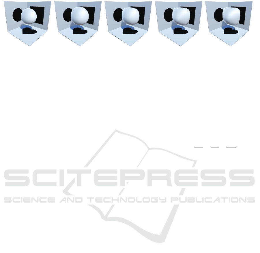
(a) 5
th
iteration. (b) 10
th
iteration. (c) 20
th
iteration. (d) 50
th
iteration. (e) 100
th
iteration.
Figure 3: Optimization process. Black shapes which are mapped onto the 3D walls are designed by the user. Figure (a-
d) shows the intermediate results generated through the optimization process. During the process, as the cost values are
decreasing, the isosurface of the NURBS volume is improving progressively to match with the user’s design. Figure (e)
shows the result of the finally optimized NURBS volume. As we can see, the result is similar to the user’s input.
weights set for shape cost and smooth cost respec-
tively. We empirically set a larger smooth cost weight
w
smooth
= 0.9 and smaller shape cost w
shape
= 0.1 for
achieving a better result. More details of shape cost
and smooth cost are discussed in later subsections.
Shape Cost Function. As one of the most impor-
tant costs for shape matching optimization, the shape
cost function is always used for evaluating how many
differences there are between the synthesized shape
and the target shape. Let 2D binary scalar field func-
tion x(u, v), y(w,u), and z(w, v) are interpolated from
the binary shape images defined by the user for top
view, left view and front view respectively. Noted
that after the 2D interpolation, these binary scalar
fields parameter space (u,v, w) are consistent with the
NURBS volume scalar field function f (u,v, w) that
we want to optimize. As we want the optimized
NURBS volume to satisfy all three views, we need
to use multiplication to achieve the effects of Boolean
AND operation. Therefore, we calculate the shape
cost through the volumetric integral of the differ-
ence between the multiplication of the binary shapes
g(u,v,w) and the NURBS volume f (u, v,w) within the
parameter space. The shape cost is calculated as:
C
shape
( f ) =
ZZZ
V
|g(u,v,w) − f (u,v,w)|
2
dudvdw,
(2)
where g(u,v, w) = x(u,v)y(w,u)z(w, v) and the volu-
metric parameters u,v,w ∈ [0,1].
Smooth Cost Function. In order to generate a
smooth volumetric NURBS field, we penalize the
rapid changes that happened to the volumetric field
in the nearby area at an arbitrary position. Here,
we introduced the Laplace operators (∇
2
) to calcu-
late the sharpness of volumetric NURBS scalar field
f (u,v,w). By minimizing the volumetric integral of
the divergence (∇·) of the gradient (∇) of the volu-
metric NURBS scalar field, we will have the entire
volumetric field as smooth as possible. The smooth
cost C
smooth
is represented as:
C
smooth
( f ) =
ZZZ
V
∇
2
f (u,v,w)dudvdw, (3)
where the volumetric parameters u,v, w ∈ [0,1] and
the Laplace operator (∇
2
) for three dimensions co-
ordinates (u,v,w) is given by the sum of the second
partial derivatives for both u, v, and w which is:
∇
2
f (u,v,w) =
∂
2
f
∂u
2
+
∂
2
f
∂v
2
+
∂
2
f
∂w
2
(4)
Optimization Process. We use L-BFGS (Limited-
memory BFGS) (Liu and Nocedal, 1989) to op-
timize the NURBS volume. L-BFGS is an
optimization algorithm in the family of quasi-
Newton methods that approximates the Broy-
den–Fletcher–Goldfarb–Shanno algorithm (BFGS)
using a limited amount of computer memory. Ac-
cording to the total cost function of the NURBS vol-
ume C
total
( f ) described in Equation 1. L-BFGS can
automatically find the gradient of the total cost func-
tion ∇C
total
( f ) and update those control values and
control weights according to the gradients. Repeating
this process until the maximum number of iterations
is reached, the NURBS volume is optimized. In L-
BFGS, for each iteration step, there is an approximate
Hessian matrix and a search direction solved from the
gradient. Iteration step size is solved through a one-
dimensional optimization (line search), then the up-
dates are the search direction multiplied by the step
size. These optimization steps are applied several
times until a local minimal solution is found or the
maximum number of iterations is reached.
As shown in Figure 3, the NURBS volume is fine-
tuned automatically with an L-BFGS optimizer. Dur-
ing the optimization process, the control values and
control weights of the NURBS volume are corrected
step by step through the L-BFGS optimization algo-
rithm without any user interactions. As we can see
from the subfigures, the optimization algorithm con-
verges pretty fast and get quite satisfying result within
Multi-view NURBS Volume
231
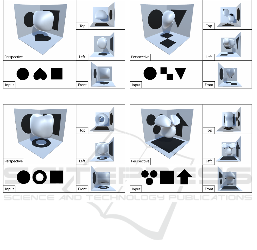
(a) User input 1: circle, heart, and square. (b) User input 2: circle, blocks, and triangle.
(c) User input 3: circle, ring, and square. (d) User input 4: dots, square, and arrow.
Figure 4: Experimental results of multi-view volumetric NURBS generated with different user inputs. In this figure, we
present the visual effects when applying different types of user input of shapes that are defined for different view directions. In
subfigure (a-d), they present four different volumetric NURBS isosurfaces generated with our proposed optimization approach
according to four different user inputs. As we can see, most results can match the input shapes on different views accordingly.
the first 50 iterations. In this example, we set the max-
imum number of iterations as 100 and the result is vi-
sually acceptable in the end.
5 EXPERIMENTAL RESULTS
Implementations. We have implemented the pro-
posed multi-view volumetric NURBS design inter-
face using Unity 3D with the 2019 version. Our
proposed L-BFGS optimization algorithm is imple-
mented in MinGW C++ using the StanMath and
Eigen library. The hardware configurations contain
Intel Core i5 CPU, 32GB DDR4 RAM, and NVIDIA
GeForce GTX 1650 4GB GDDR6 Graphics Card.
Changing User Inputs. We tested our optimiza-
tion approach on generating multi-view volumetric
NURBS with respect to different user inputs. As
shown in Figure 4, four different volumetric NURBS
isosurfaces are generated with our proposed optimiza-
tion approach according to four different user inputs.
All examples are generated with same parameter set-
tings: control order o = 3, ctrl size m = n = l = 50,
cell size is 20 × 20 × 20 and the max optimization it-
erations are 100. For each iteration, it typically takes
about 4 sec. Overall, all of the examples are typically
generated with about 400 sec. Those isosurfaces ex-
tracted from the optimized NURBS volumes in these
examples are set up with an isovalue of C = 0.5.
Generally speaking, most of the results demon-
strated here are seeming to match with the user’s in-
put shapes from different view directions. For exam-
ple, the front view in (a) looks like a square exactly,
the front view in (b) looks pretty much like a trian-
gle, the top view in (c) looks like a circle as is ex-
pected, and the left view in (d) shows three dots there
GRAPP 2022 - 17th International Conference on Computer Graphics Theory and Applications
232
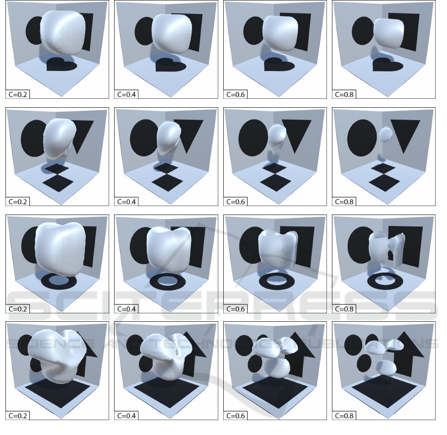
Figure 5: Experimental results of changing isovalues. In this figure, we present the visual effects of applying different
isovalues when extracting isosurfaces on the same optimized NURBS volumes. Four different rows present four different
volumetric NURBS optimized from the four user inputs specified in Figure 4 with the parameters settings claimed earlier.
Four different columns demonstrate four different isosurfaces for each NURBS volume given four isovalues settings, they
are C =0.2, 0.4, 0.6, and 0.8 respectively. As we can see there is a trend that as the isovalue C grows higher, the shape of
isosurfaces shrinks. Therefore, we need to find a balance point to best describe the optimized NURBS volume. According to
the empirical experiences, typically C ∈ [4.5,5.5] results in better visual effects.
clearly. But there are some imperfections in some
view directions such as the left view in (a) and (b)
look not like a perfect circle and the top view in (d)
is not a square and the front view in (d) does not look
like an arrow. This can be explained as we hope to
ensure the smoothness in the generated NURBS vol-
umes, therefore, low-level details such as sharp edges
on the arrow will disappear automatically. We will
discuss more about how to improve the result’s qual-
ity through precision control in a later experiment.
Changing Isovalues. We conducted numerical exper-
iments to test the visual effects of changing isovalue C
when extracting the isosurface in optimized NURBS
volume fields f
∗
(u,v,w) = C. As shown in Figure 5,
different isovalue results in different isosurfaces re-
sults. In overall, there is a trend that higher isovalue
results in a thinner shape of isosurfaces. For example,
as shown in the last example in the figure, when we set
Multi-view NURBS Volume
233
(a) Lower control precision. (b) Higher control precision.
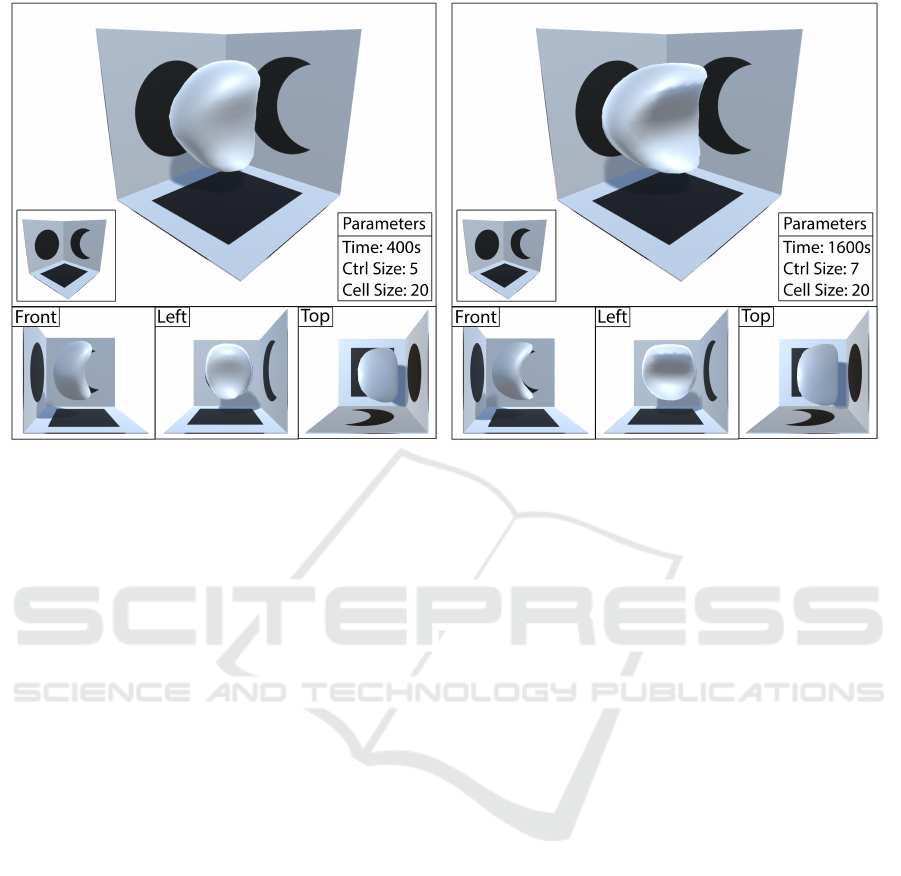
Figure 6: Experimental results of improving control precision. This figure shows a comparison result between (a) lower
control precision and (b) higher control precision. In (a) the control size is m = n = l = 5 while in (b) the control size is
m = n = l = 7. Both result isosurfaces are extracted with the same cell size 20 × 20 × 20 and same isovalue C = 0.5. As we
can see there are differences in the detail of the shape between different levels of precision control. In (b) with higher control
degrees, the shape of the moon in the front view matches better than (a) which is generated with lower control degrees.
C = 0.2, the isosurface is too fat to see three dots any-
more, but when we set C = 0.8 the isosurface is too
skinny so that there are only three dots (spheres) left.
Most experiments’ results follow the rule that mod-
erate isovalues settings result in acceptable visual ef-
fects that are neither too fat nor too skinny. Typically
a balance point C ∈ [4.5,5.5] can best describe the op-
timized NURBS volume which are matching with the
user’s input shapes pretty well.
Improving Control Precision. As pointed out ear-
lier, low precision control over the optimized NURBS
volume will cause a loss of low-level details in the re-
sulting isosurface such as the sharp edges defined in
the shapes drawn by users. Here we discuss more de-
tails about improving the control precision. As shown
in Figure 6, results on two different levels of con-
trol precision are presented. (a) shows a result with
a smaller precision control size which is 5. While
(b) shows a higher precision control size which is 7.
Therefore, the difference between the two control lev-
els are 7
3
−5
3
= 218 and there is a 218/5
3
= 74% in-
crease over the control degree. As we can see, higher
control precision results in an isosurface with more
levels of geometric details. For example, from the
front view, (a) shows a moon-like shape that is fatter
in middle and there is no sharp corner at two end-
ing points. But from (b), we can see a more realistic
moon shape which has a thinner middle part but with
sharper corners at two ends. We appreciate such an
improvement in the quality of the result, but the price
is the three times more seconds spent on optimizing a
NURBS volume with higher control precision.
Missing Smoothness Control. In our proposed opti-
mization algorithm, by default, we enforce a smooth-
ness consideration on the optimized NURBS vol-
umes. Let us explore what happens if we turn off the
smooth cost and ignore the smoothness control. As
shown in Figure 7, (a) a rough isosurface extracted
from the NURBS volume optimized without smooth
cost and (b) a smooth isosurface extracted from the
NURBS volume optimized with smooth costs turned
on are presented. As we’d prefer to generate smoother
results, therefore, the smooth cost is a very important
factor need to be considered during the optimization.
Failure Cases. During the experiments, we realize
there are lots of settings that result in failure cases.
First, the control size can not be too small, e.g., 1, 2,
3, ... In these cases, the NURBS volume can not be
optimized at all and results in some random NURBS
values. It also fails when cell size is too high, say, 25
3
.
In this case, no isosurface can be extracted from the
NURBS volume. If the control size is too large, say
m = n = l = 10, no enough memory space is available
for such a high space-demanding computational task.
GRAPP 2022 - 17th International Conference on Computer Graphics Theory and Applications
234
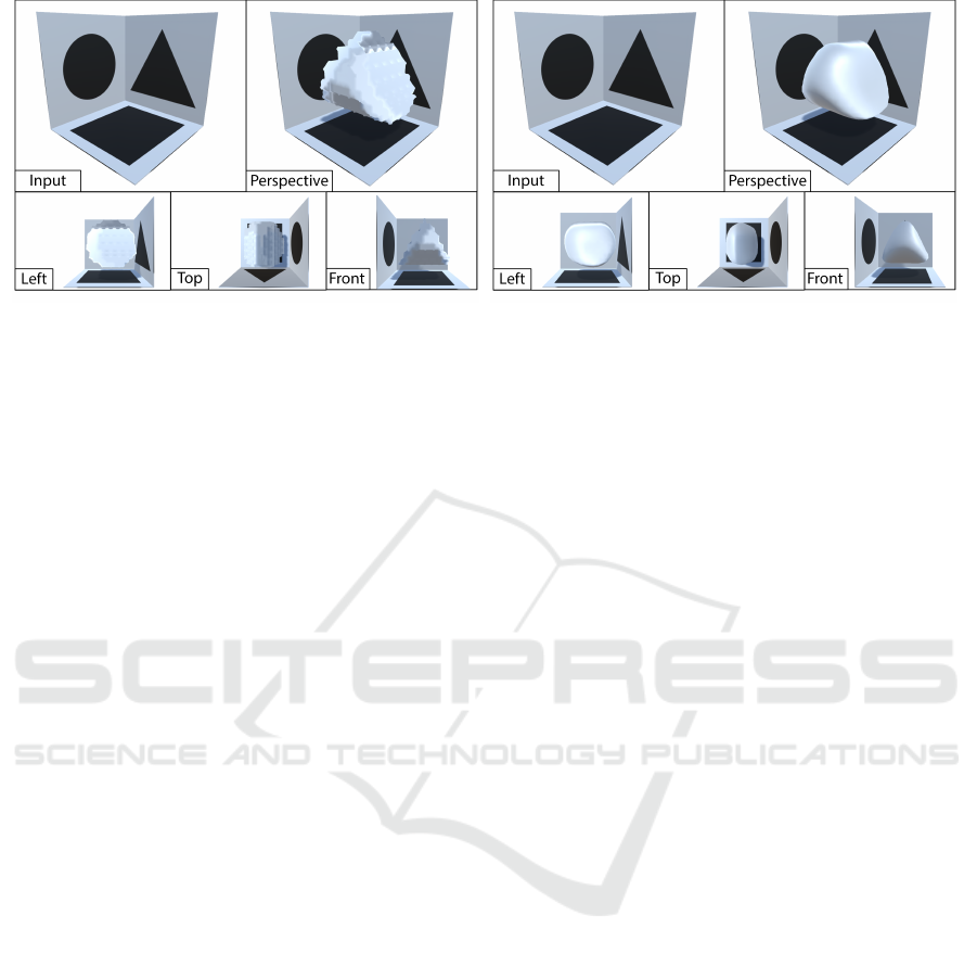
Figure 7: Experimental results of missing smoothness control. This figure shows a comparison result between (a) without
smooth cost and (b) with smooth cost. Both in (a) and (b) shares the same control size of m = n = l = 5 and their result
isosurfaces are extracted with the same cell size 20 × 20 × 20 and same isovalue C = 0.5. As we can see, (a) shows a rough
surface where there are lots of abrupt changes along the edges in the NURBS volume, while (b) shows a smooth surface where
the NURBS volume has smoother distributions over its NURBS field.
6 CONCLUSIONS
In this paper, we present a novel interface for multi-
view NURBS volume geometric modeling. We de-
vise an optimization algorithm to automatically re-
construct the 3D NURBS volume which is match-
ing with user’s designs from different view directions.
Through a series of results, we show that our proposed
approach can reconstruct the NURBS volume that
matches with the user’s designs. At the same time,
we conclude that moderate isovalue settings, smooth-
ness considerations, and higher control precision will
result in better results. But higher precision needs ex-
tra time for optimization. We believe our work can
inspire more follow-up research to explore how the
volumetric NURBS design can change the industry
of the CAD and graphics industry.
REFERENCES
Aleotti, J., Caselli, S., and Maccherozzi, G. (2005). Tra-
jectory reconstruction with nurbs curves for robot
programming by demonstration. In 2005 Interna-
tional Symposium on Computational Intelligence in
Robotics and Automation, pages 73–78. IEEE.
Fuhrmann, S., Langguth, F., and Goesele, M. (2014). Mve-
a multi-view reconstruction environment. In GCH,
pages 11–18. Citeseer.
Hashemian, A. and Hosseini, S. F. (2018). An integrated
fitting and fairing approach for object reconstruction
using smooth nurbs curves and surfaces. Computers
& Mathematics with Applications, 76(7):1555–1575.
Hsiao, K.-W., Huang, J.-B., and Chu, H.-K. (2018). Multi-
view wire art. ACM Trans. Graph., 37(6):242–1.
Imani, B. and Hashemian, S. A. (2012). Nurbs-based
profile reconstruction using constrained fitting tech-
niques. Journal of Mechanics, 28(3):407–412.
Labatut, P., Pons, J.-P., and Keriven, R. (2007). Efficient
multi-view reconstruction of large-scale scenes using
interest points, delaunay triangulation and graph cuts.
In 2007 IEEE 11th international conference on com-
puter vision, pages 1–8. IEEE.
Lavoie, P., Ionescu, D., and Petriu, E. (1999). A high pre-
cision 3d object reconstruction method using a color
coded grid and nurbs. In Proceedings 10th Interna-
tional Conference on Image Analysis and Processing,
pages 370–375. IEEE.
Liu, D. C. and Nocedal, J. (1989). On the limited memory
bfgs method for large scale optimization. Mathemati-
cal programming, 45(1):503–528.
Pal, P. (2008). A reconstruction method using geomet-
ric subdivision and nurbs interpolation. The interna-
tional journal of advanced manufacturing technology,
38(3):296–308.
Saini, D., Kumar, S., and Gulati, T. R. (2015). Reconstruc-
tion of free-form space curves using nurbs-snakes and
a quadratic programming approach. Computer Aided
Geometric Design, 33:30–45.
Saini, D., Kumar, S., Singh, M. K., and Ali, M. (2021).
Two view nurbs reconstruction based on gaco model.
Complex & Intelligent Systems, pages 1–18.
Sinha, S. N. and Pollefeys, M. (2005). Multi-view recon-
struction using photo-consistency and exact silhou-
ette constraints: A maximum-flow formulation. In
Tenth IEEE International Conference on Computer
Vision (ICCV’05) Volume 1, volume 1, pages 349–
356. IEEE.
Vu-Bac, N., Duong, T. X., Lahmer, T., Zhuang, X., Sauer,
R. A., Park, H., and Rabczuk, T. (2018). A nurbs-
based inverse analysis for reconstruction of nonlinear
deformations of thin shell structures. Computer Meth-
ods in Applied Mechanics and Engineering, 331:427–
455.
Zhong, D., Liu, J., Li, M., and Hao, C. (2008). Nurbs recon-
struction of digital terrain for hydropower engineer-
ing based on tin model. Progress in Natural Science,
18(11):1409–1415.
Multi-view NURBS Volume
235
