
Univariate Time Series Prediction using Data Stream Mining
Algorithms and Temporal Dependence
Marcos Alberto Mochinski
a
, Jean Paul Barddal
b
and Fabrício Enembreck
c
Graduate Program in Informatics, PPGIa, Escola Politécnica, Pontifícia Universidade Católica do Paraná, PUCPR
Curitiba, Brazil
Keywords: Time Series Forecasting, Data Stream Mining Algorithms, Multiple Time Series, Ensemble, Feature
Engineering, Temporal Dependence.
Abstract: In this paper, we present an exploratory study conducted to evaluate the impact of temporal dependence
modeling on time series forecasting with Data Stream Mining (DSM) techniques. DSM algorithms have been
used successfully in many domains that exhibit continuous generation of non-stationary data. However, the
use of DSM in time series is rare since they usually are univariate and exhibit strong temporal dependence.
This is the main motivation for this work, such that this study mitigates such gap by presenting a univariate
time series prediction method based on AdaGrad (a DSM algorithm), Auto.Arima (a statistical method) and
features extracted from adjusted autocorrelation function (ACF) coefficients. The proposed method uses
adjusted ACF features to convert the original series observations into multivariate data, executes the fitting
process using the DSM and the statistical algorithm, and combines the AdaGrad's and Auto.Arima's forecasts
to establish the final predictions. Experiments conducted with five datasets containing 141,558 time series
resulted in up to 12.429% improvements in sMAPE (Symmetric Mean Average Percentage Error) error rates
when compared to Auto.Arima. The results depict that combining DSM with ACF features and statistical time
series methods is a suitable approach for univariate forecasting.
1 INTRODUCTION
To work with univariate time series, the information
available for the prediction must be extracted from
the series’ observations. A series can be summarized
in a set of events observed in time at a constant
frequency (Makridakis, 1976). Statistical algorithms,
such as regression algorithms, identify the temporal
dependencies between the elements of a series. Yet,
this is not a characteristic inherent to all data stream
mining (DSM) algorithms that are multivariate in
nature, i.e., to deal with univariate data they depend
on attributes (artificial or not) to improve their
learning mechanism.
In time series, the temporal dependence between
the series' observations can be identified by analyzing
the correlation between the elements of the series,
called autocorrelation. Autocorrelation expresses the
correlation between an observation of the series and
a
https://orcid.org/0000-0002-7118-9993
b
https://orcid.org/0000-0001-9928-854X
c
https://orcid.org/0000-0002-1418-3245
its lagged values (Hyndman, 2014). This paper
proposes the extraction of features from
autocorrelation function (ACF) and the combination
of DSM algorithms with univariate autoregressive
models in multi-series scenarios. We show that using
time dependency features improves AdaGrad's
(Duchi et al., 2011) predictions, and their
combination with Auto.Arima's (Box and Jenkins,
1976) predictions yields lower error rates.
The main motivation for this study is that the use
of DSM algorithms in univariate time series
prediction is rare, since time series usually present
strong temporal dependence and they are constituted
solely by their observed values. Although in a
previous paper (Mochinski et al., 2020), DSM has
been applied to time series forecasting, the impact of
temporal dependency modeling in this context is
unexplored so far. Thus, proposing a novel method
focusing on this scenario is challenging. In our
398
Mochinski, M., Barddal, J. and Enembreck, F.
Univariate Time Series Prediction using Data Stream Mining Algorithms and Temporal Dependence.
DOI: 10.5220/0010859600003116
In Proceedings of the 14th International Conference on Agents and Artificial Intelligence (ICAART 2022) - Volume 2, pages 398-408
ISBN: 978-989-758-547-0; ISSN: 2184-433X
Copyright
c
2022 by SCITEPRESS – Science and Technology Publications, Lda. All rights reserved

approach, we opted for the use of adjusted ACF
coefficients as new features for the univariate time
series processing and we explore its applicability in
an extensive experimentation process using series of
different datasets.
First, we discuss related works on time series
forecasting and the use of temporal dependence in
different scenarios. Next, we introduce our approach
for the feature engineering process and the method
used to evaluate it, which is later analyzed in the
following section. Finally, we conclude this paper and
list future works.
2 RELATED WORK
Authors in (Žliobaitė et al., 2015) cite that temporal
dependence can also be called serial correlation or
autocorrelation and explain that in data stream
problems, an input set of multi-dimensional variables
submitted to a DSM algorithm usually contains the
information that makes it possible to process the data
classification or prediction. They discuss that the past
values of the target variable (usually the only
information available for univariate data) are not
enough for the predictive process.
According to (Stojanova, 2012), there are four
different types of autocorrelation: spatial, temporal,
spatio-temporal and network (relational)
autocorrelation. Stojanova explains that spatial
autocorrelation is defined as the correlation among
data values that considers their location proximity.
Therefore, near observations are more correlated than
distant ones. Temporal autocorrelation refers to the
correlation of a time series with its own past and
future values, and the author cites that it can be also
called lagged correlation or serial correlation, as in
(Žliobaitė et al., 2015). Spatio-temporal
autocorrelation considers spatial and temporal
correlation between observations, and network
autocorrelation expresses the interdependence
between values in different nodes of a network.
In this paper we focus on temporal
autocorrelation. Authors in (Stojanova, 2012) explain
that temporal autocorrelation is the simplest form of
autocorrelation as it focuses on a single dimension,
i.e., time. Many fields study autocorrelation. Authors
in (Nielsen et al., 2018) use autocorrelation to predict
the wave-induced motion of a marine’s vessel by
combining values of autocorrelation function and
previous measurements. Despite the fact that the
autocorrelation can express a stationary condition, the
authors use a sample of an ACF (autocorrelation
function) obtained at a recent time window to help in
the prediction of a dynamic system, considering that
the values are valid as they have not changed
significantly. The authors cite in (Nielsen et al., 2018)
that the ACF function can be seen as a direct
measurement of the memory effect of a physical
process.
Authors in (Rodrigues and Gama, 2009) use
autocorrelation coefficients in an electricity-load
streams prediction study. They identify the
correlation of historical inputs and use the most
correlated values as input to a Kalman filter system
used in combination with a multi-layered perceptron
neural network to create new predictions across
different horizons, i.e., one hour, one day, and one
week ahead load forecasts.
Authors in (Duong et al., 2018) used temporal
dependencies to detect changes in streaming data.
The authors introduce a model named Candidate
Change Point Detector (CCPD), used to model high-
order temporal dependencies and compute the
probabilities of finding change points in the stream
using time dependency information from different
points of the stream.
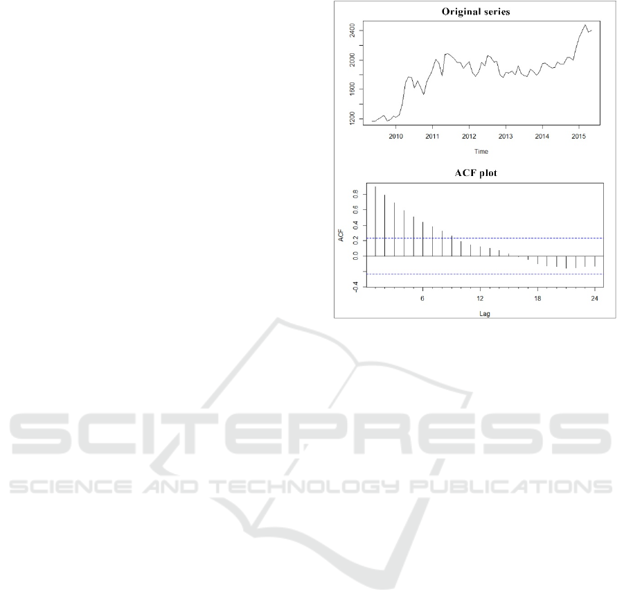
According to (Hyndman, 2014), autocorrelation
measures the linear relationship between lagged
values of a time series. Figure 1 presents the original
data for a time series and its ACF (autocorrelation)
function plot. The authors in (Hyndman, 2014)
explain that, in an ACF plot, the relationship r
k
expressed between two events
y
t
and y
t-k
can be
written as follows (1):
(1)
where T represents the length of the time series in
analysis, and
ȳ the mean of its observations. Authors
also inform that trend and seasonality can also be
evaluated from the analysis of the ACF plot: trend
data tend to have positive values that slowly decrease
as the lags increase; seasonal data, on the other hand,
will present larger values for the autocorrelation
coefficients at multiples of the seasonal frequency.
According to (Werner and Ribeiro, 2003), ACF
functions evaluate the stationarity of a series. In
general, when analysing an ACF plot, it is important
to observe the coefficients that present most
significant values (statistically different from zero).
As described previously in this paper, a time
series is defined as a set of events observed in time at
a constant frequency (Makridakis, 1976). In (Esling
and Agon, 2012), authors complement that a time
series can be defined as a set of contiguous instants of
time, and that a series can be univariate or
Univariate Time Series Prediction using Data Stream Mining Algorithms and Temporal Dependence
399
multivariate (when several series simultaneously
cover several dimensions in the same time interval).
In general, it can be said that a univariate series is one
whose observations refer to a single variable, and a
multivariate series is one that contains information
relating to more than one variable. In this work, we
present a prediction approach for multi-series
scenarios where a set of univariate time series is
available, regardless of whether these are inter-
correlated or not. Our approach is multivariate
because, at first, it converts original univariate series
observations into multivariate data using adjusted
ACF coefficients as their additional features.
Despite the exciting results of classical statistical
methods for time series forecasting, it is increasingly
common to find machine learning alternatives, or
even their combination. Modern techniques like data
stream mining (DSM) algorithms deal with big data
scenarios or situations in which it is inconceivable, or
at least difficult, to have access to the entire dataset at
once. The authors in (Bontempi et al., 2013) say that,
in the last two decades, machine learning models have
established themselves as serious competitors to
classical statistical models. This study, in turn,
proposes the combined use of a classical statistical
method and a DSM algorithm to benefit from their
characteristics.
The authors in (Bifet et al., 2018) enumerate,
among other characteristics, that a data stream mining
algorithm must process one instance at a time using a
limited amount of memory and time for processing,
and that it must be able to give a response at any time,
detecting and adapting a model to temporal changes.
Modern applications demand faster responses and
innovative techniques that adapt to the increasingly
overloaded world of information in which we live.
According to (Gama et al., 2014), learning should
take place in an incremental and adaptive fashion,
thus allowing the reaction to variations in data
behaviour (concept drifts) and the data prediction in
an increasingly precise way. It is essential that the
algorithms used in time series analysis can identify
variations of data behaviour with greater accuracy so
that the forecasting process is more precise. Thus, it
is justifiable to seek to apply data stream mining
algorithms, which allow gradual, incremental
processing of the observations, and which are highly
adaptive in time series forecasting. In this work,
statistical and DSM algorithms forecasts are
combined to improve their individual results.
AdaGrad (Duchi et al., 2011) is an example of an
adaptive data stream mining algorithm, capable of
dealing with very sparse and non-sparse data.
Figure 1: M1 series (M4 dataset). Original data and ACF
plot. Dotted lines in the ACF plot indicate the confidence
interval. We may consider the values inside this interval as
not statistically significant.
According to the authors in (Duchi et al., 2011),
AdaGrad generalizes the online learning paradigm of
specializing an algorithm to fit a particular dataset,
and automatically adjusts the learning rates for online
learning and stochastic gradient descent on a per-
feature basis.
Regarding statistical algorithms for time series
forecasting, this work focuses on the use of
Auto.Arima (Hyndman and Khandakar, 2008;
Hyndman et al., 2019), an automated implementation
of ARIMA (Box and Jenkins, 1976), a classic
statistical algorithm also known as a Box-Jenkins
model. In a problem with multiple time series, to
avoid demanding an individual analysis of each
series, a solution that automates the selection of the
best ARIMA parameters can certainly be of great help
in the process. Therefore, we seek to predict multiple
time series without the need for a meticulous analysis
of each series, thus rendering the process user-
independent.
The combined use of different algorithms is not a
novelty in time series forecasting. In competitions
like M4 (Makridakis et al., 2018a), from the 17 most
accurate results, 12 used combinations and one used
a hybrid approach integrating statistical and machine
learning methods.
Authors in (Mochinski et al., 2020) also explore
using a hybrid approach combining DSM and
statistical algorithms in univariate time series
ICAART 2022 - 14th International Conference on Agents and Artificial Intelligence
400

prediction. The proposed method executes the fitting
process using a DSM algorithm and Auto.Arima, and
selects the best algorithm for the series' forecasting
based on the calculated fitting error. We think that
using a different technique can improve the feature
engineering process used by that study. Based on this
assumption, we decided to extend it by using the
temporal dependence information present on each
series for the feature engineering. For this, we
decided to explore the Temporally Augmented
concept (presented in (Žliobaitė et al., 2015) for
classification problems) and the use of ACF
coefficients as the basic information for the creation
of additional features for time series processing. To
validate our proposal, we applied it to a more diverse
set of time series, resulting in more extensive
experimentation than that observed in (Mochinski et
al., 2020). For data stream mining algorithms, an
additional issue being considered is their dependence
on multivariate input vectors capable of helping their
learning process. This is handled in our proposal by
introducing time dependence features as their input.
3 THE AA-ACF METHOD FOR
TIME SERIES FORECASTING
In this section, we describe the Auto.Arima and
AdaGrad Autocorrelation Coefficient Function (AA-
ACF) method, which is the result from an exploratory
study conducted to evaluate the combined use of
statistical and DSM methods for improved univariate
time series forecasting.
The proposed method includes the following
phases: pre-processing, training, algorithm selection
and forecasting. In the pre-processing phase, the time
series data is loaded, and the feature engineering
process is done. In the training phase, Auto.Arima
and AdaGrad are trained and assessed w.r.t. training
error. The algorithm selection phase picks the
algorithm that presented the lowest training error, and
finally, in the forecasting phase the predictions for the
time series are calculated using the algorithm selected
to each series. Our implementation was created using
the R language, which also controls the execution of
the MOA framework (Bifet et al., 2010), where
AdaGrad training and forecasting are done. Details
about each step of the proposal are given below.
1
The use of 288 observations (W288) and 18 lags are
explained in detail in the "AA-ACF hyperparameters"
subsection.
3.1 Pre-processing
To introduce the concept of temporal dependence on
the series attributes, coefficients obtained with the
autocorrelation function (ACF) are extracted from the
series and used in the creation of new features.
Considering the nature of DSM algorithms, which
do not analyze all data in batch mode since they work
with the most recent instances of the series, the
concept of a sliding window was used. Also, the use
of this technique allows for the adjustment of the
autocorrelation coefficients during the entire feature
engineering process, adapting them to the most recent
aspect of the series events.
In the feature engineering process, the additional
attributes associated with each observation in the
series are created based on previous events (values
from previous observations in the series), using
sliding windows of up to 288 observations (referred
in this study as W288). The window data is used to
calculate ACF coefficients that express the
relationship between an observation and the events
that precede it.
The coefficients generated for the first 18 lags
1
are considered as the most relevant for the purpose of
this approach in spite of their values, i.e., positive and
negative values are considered. The rationale behind
using time dependency attributes in the feature
engineering process was based on the study of
(Žliobaitė et al., 2015), which proposed the use of
temporal autocorrelation in data stream classification
problems. For classification, it suggests two
approaches: the Temporal Correction classifier in
which the predictive model is adapted to support the
concept, and the Temporally Augmented classifier,
which proposes the feature engineering process with
the advantage of not requiring modifications to the
classifier structure and, thus, allowing the use of any
algorithm, without the need to recode it.
In this paper, the Temporally Augmented concept
is adapted for regression problems of univariate
series. The goal is to create features that represent the
dependency between the input features and past
observations of each series, using them as input for
the DSM algorithms predictions. Figure 2 presents
the approach used in this study to create features
based on ACF coefficients values. The diagram
presents the creation of features for a specific time
series, and Algorithm 1 explains the process in more
detail. First, the events are read using a sliding
Univariate Time Series Prediction using Data Stream Mining Algorithms and Temporal Dependence
401
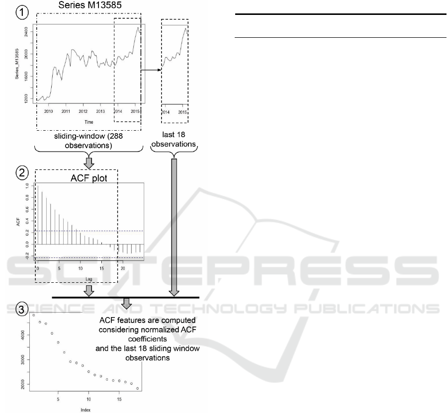
window of up to 288 registers (W288). Second, ACF
coefficients are calculated considering the events
selected in W288.
Figure 2: Feature Engineering approach diagram, based on
ACF Coefficients.
Next, the first 18 ACF coefficients are normalized
for the interval from 1 to 2 (to avoid negative or zero
values) and then multiplied for the last 18 events from
the sliding window (the most recent ones) resulting in
the ACF features (or adjusted autocorrelation
coefficients) that are added to the series. Additionally,
a feature is created based on a linear regression model
considering the W288 events. This last attribute was
created to help DSM algorithms in one-step-ahead
forecasts. It was considered necessary because of the
characteristics of the test-then-train model used by
DSM algorithms. Therefore, suggesting a more
assertive value for the next Events attribute would
help to keep DSM model calibrated, with lower error
on the prequential process.
Algorithm 1: The Feature Engineering Approach.
1: for each series in the dataset do
2: S ← series observations
// loop through each observation in the series S
// to compute its new additional features
3: for N = 1 to length(S) do
// sliding-window data (time series data type):
// select up to 288 previous events for the current
//N record in S
4: W288 ← S[N-288-1 .. N-1]
// calculate ACF coefficients for the sliding window
5: ACF_W288 ← forecast::Acf(W288, plot=FALSE)
// normalize the first 18 ACF coefficients (lags 1 to 18)
// for the range 1 to 2 to avoid negative or zero values
6: ACF_W288_norm ←
BBmisc::normalize(ACF_W288$acf[1:18],
method="range", range = c(1,2))
// select the last 18 sliding window data in reverse order
7: W288_18r ← reverse(tail(W288,18))
// multiplies normalized ACF by the last 18 values from
// the sliding window to compute the new 18 additional
// features based on ACF coefficients
8: ACF_Lag ← ACF_W288_norm * W288_18r
// create additional feature based on a linear regression
// one-step-ahead forecast considering trend and
// seasonality
9: fit ← forecast::tslm(W288 ~ trend + season)
10: fcTSLM_h1 ← forecast(fit, h=1)$mean
// new ACF_Lag1 to ACF_Lag18 and fcTSLM_h1
// features are ready to be aggregated to the original
// series data
11: S[N] ← bind(S[N], ACF_Lag1..ACF_Lag18,
fcTSLM_h1)
12: end for
// series S and its new features are stored in ARFF file
13: write series S to ARFF
14:end for
The feature engineering process creates ARFF
(Attribute-Relation File Format) files with the
following structure:
• Events (target, numeric): series observation
value.
• ACF_Lag1 to ACF_Lag18 (numeric):
features calculated based on ACF
coefficients for W288 window data,
normalized for 1 to 2 range, multiplied by
the last 18 values from the sliding window.
• fcTSLM_h1 (numeric): one-step-ahead
forecast calculated by a regression model for
W288 window (function forecast::tslm
(Hyndman et al., 2019) available for the R
language).
ICAART 2022 - 14th International Conference on Agents and Artificial Intelligence
402
AA-ACF hyperparameters:
To establish the use of 18 lagged values and
coefficients as well as to define the size of the 288-
event sliding window, previous experiments were
done using windows from 72 to 288 events, and
selecting 2, 4, 6, 12, 18, 24, 36, 48 and 60 ACF
coefficients. The final values were selected based on
the combination that presented best results, i.e., lower
sMAPE (Armstrong, 1985) values in forecasting
tests. Experiments were done using time series from
M4 dataset, selecting up to 200 series from each
periodicity (daily, hourly, monthly, quarterly,
weekly, and yearly) of that dataset, evaluating the
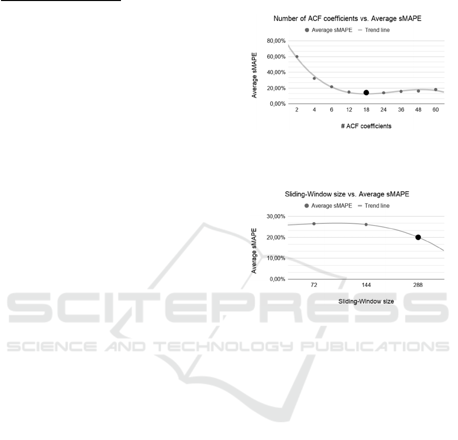
parameters in up to 1200 distinct series. The trend line
presented in Figure 3 shows that as the number of
ACF coefficients increases, lower sMAPE values are
reached considering 18 coefficients.
In Figure 4 the trend line shows that lower
sMAPE values were reached using 288-observation
sliding windows.
Naturally, the hyperparameters were set
according to the results obtained from a sample of a
specific dataset, and thus, we further analyse the
impact of this choice in a larger testbed containing
more datasets in Section 5 Results.
3.2 Training
In this step, the Auto.Arima training is done using the
function forecast::auto.arima (Hyndman and
Khandakar, 2008; Hyndman et al., 2019). For model
fitting with Auto.Arima, no additional features are
required, since only the original time series are used.
Next, the training error is calculated according to
sMAPE, depicted in (2) (cf. Section 4.3 Evaluation
Protocol). AA-ACF calculates the fitting error based
on the last n series observations (or n records, NRecs)
as depicted in Figure 5. The parameter n coincides
with the prediction horizon (h) established for the
series, based on its periodicity.
For the experiments with AA-ACF the following
prediction horizons were established: daily series,
h=14; hourly series, h=48; monthly series, h=18;
quarterly series, h=8; weekly series, h=13; annual
series, h=6.
Next, ARFF files prepared with ACF features (see
Algorithm 1) are processed with AdaGrad using the
prequential mode in MOA, and the training error
(sMAPE) is calculated based on the last n records of
the series.
3.3 Algorithm Selection
Figure 3: Results of the experiments to select the number of
ACF coefficients for the AA-ACF method. Trend line
shows lower average sMAPE value for 18 ACF
coefficients.
Figure 4: Results of the experiments to select the size of the
sliding-window for the AA-ACF method. Trend line shows
lower average sMAPE value for a 288-observation sliding-
window.
Algorithm selection is performed based on the
training error (sMAPE) obtained for each algorithm
(Auto.Arima and AdaGrad) in the training phase. The
algorithm that presented the smallest error is selected
for each series forecasting.
3.4 Forecasting
AA-ACF implements three strategies to forecast a
series according to the option selected by the user.
The first strategy is called SelectionNRecs (or simply
NRecs) and consists of selecting the algorithm based
on the training error computed on the last n records of
the series and calculating the series forecasts using
the algorithm that presented smallest training error.
The second strategy (default) is called
SelectionAndFusion (or Fusion), which also consists
of selecting the algorithm given the error calculated
during the training phase. Next, if the algorithm
selected for the series is Auto.Arima, forecasting
values are calculated using this algorithm. Else, if the
Univariate Time Series Prediction using Data Stream Mining Algorithms and Temporal Dependence
403
selected algorithm is AdaGrad, the forecasts
calculated using AdaGrad will be combined with the
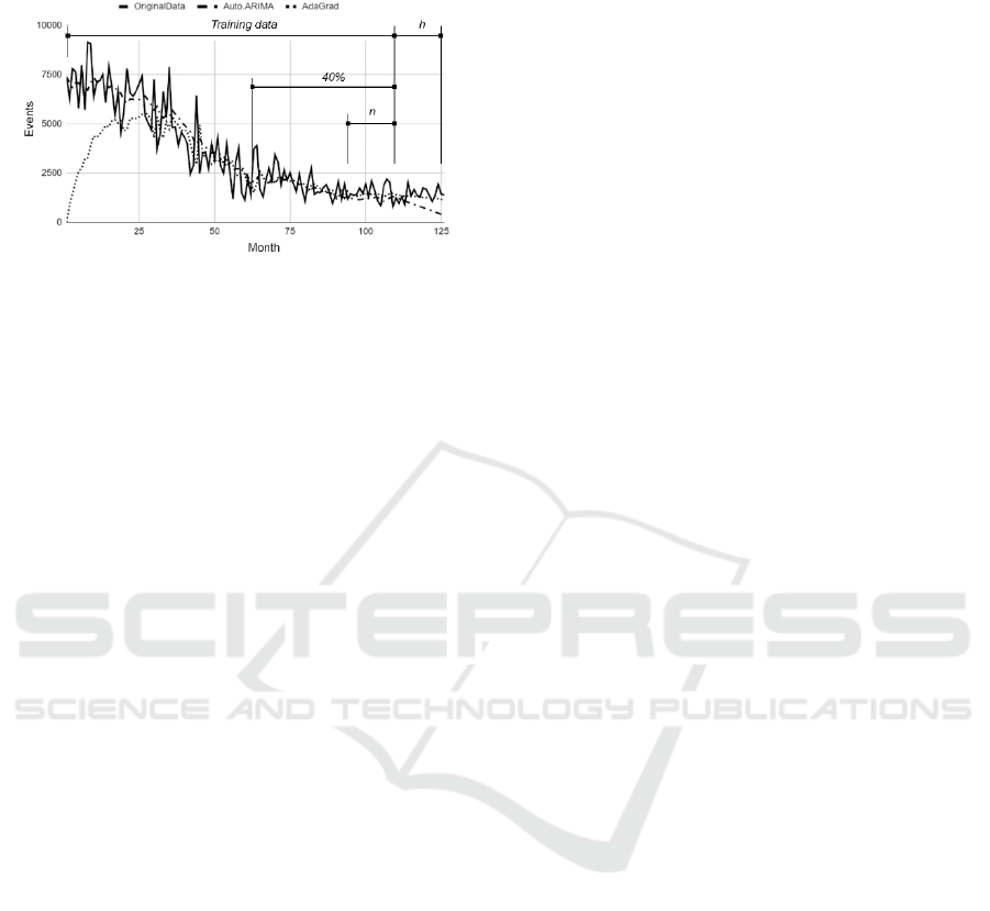
Figure 5: Original data from the N1738 time series (M3
dataset) and values obtained in the training and forecasting
by AdaGrad and Auto.Arima (h=forecasting horizon).
“40%” and “n” indicate portions considered in the fitting
error calculation.
Auto.Arima forecasts using a fusion process based on
the average of the forecasts of both methods.
The third strategy is called Selection40p (or 40p).
It is similar to the NRecs strategy, however, instead
of calculating the training error based on the last n
records of the series, the last 40% of the records are
considered.
For the Auto.Arima forecasting, the function
forecast::auto.arima is used to establish the fitting
model, and the function forecast::forecast to calculate
the h forecasts (h=prediction horizon) for the series
being analysed. For AdaGrad forecasting, ARFF files
prepared with ACF features (see Algorithm 1) are
used. A program in R is used to control the iterative
process of the execution of the streamer and get its
one-step-ahead forecasts. After obtaining the forecast
for one horizon, the ACF feature engineering process
is considered to prepare a file for the next prediction,
until the forecasting horizon (h) is reached. The
process is repeated from 6 to 48 times for each series
according to its periodicity.
4 EXPERIMENT
The experiment carried out in this study aimed at
validating the hypothesis that a DSM algorithm used
in combination with a statistical method presents
competitive results with those obtained by a classic
statistical method. Besides the combined use of
algorithms, the evaluated method proposes the use of
additional features that are able to represent temporal
dependency characteristics, capable of expressing or
translating the temporal profile of the series as input
to the learning process.
It is important to say that this study is part of an
extensive work that evaluated in previous phases the
use of different DSM algorithms available in MOA,
and selected AdaGrad based on its results. Regarding
statistical algorithms, ARIMA was chosen as a
classical method applicable to a wide range of series
prediction problems, and selected among other
statistical methods based on its results in earlier
studies for the feature engineering process that
evaluated its use and other statistical methods
available as functions of the forecast package
(Hyndman et al., 2019) available for R.
The forecast::auto.arima function was selected as
the statistical algorithm used in this study given its
ability to automatically select its parameters and
because of its use in metalearning methods like those
proposed in (Montero-Manso et al., 2018a; Montero-
Manso et al., 2018b), that use Auto.Arima combined
with a set of different algorithms.
This section is organized with the following
subsections: Algorithms and Tools, Datasets, and
Evaluation Protocol.
4.1 Algorithms and Tools
To perform the experiment, the following algorithms
and tools were mainly considered:
1) Statistical algorithm: forecast::auto.arima
(Hyndman and Khandakar, 2008).
2) Data stream mining algorithm: AdaGrad (Duchi
et al., 2011). Hyperparameters:
learningRate=0.01, epsilon=1e-8,
lambdaRegularization=0, lossFunction=HINGE.
3) Tools:
a) MOA (Massive Online Analysis): a
framework for data stream mining (Bifet et al.,
2010).
b) R language (R Core Team, 2018) and RStudio
(RStudio Team, 2020): programming
language R and IDE for R programming.
c) Main R packages: Metrics (Hamner and
Frasco, 2018), forecast (Hyndman and
Khandakar, 2008), and BBmisc (Bischl et al.,
2017).
4.2 Datasets
The experiments were performed using 141,558
univariate time series available in 5 different datasets
described as follows:
Dataset 1 (M3 competition, 3003 time series):
The M3 dataset is composed of 3003 time series from
the M3 competition (Makridakis and Hibon, 2000).
The dataset includes series with monthly, yearly,
ICAART 2022 - 14th International Conference on Agents and Artificial Intelligence
404

quarterly, and other periodicities, with data extracted
from different domains, like Macroeconomics,
Microeconomics, Demographic data among others.
In this dataset the series are relatively short, with
lengths ranging from 14 to 126 events. Therefore, it
is a dataset that can help to evaluate the behaviour of
the AA-ACF method in short series.
Dataset 2 (M4 competition, 100,000 time
series): The M4 dataset has a set of 100,000
differently ranged time series (13 to 9,919
observations) used in the M4 competition
(Makridakis et al., 2018a). In the M4 dataset, the
series represent information from different domains
such as Microeconomic, Macroeconomic,
Demography data, among others, making it possible
to verify the applicability of the proposed method for
data of different domains, with different profiles,
some showing a higher level of data variation, while
others may have a linear trend, without major
variations in terms of seasonality and trend.
Dataset 3 (M5 competition, 30,490 time series):
The M5 dataset contains time series data from
product sales of a large supermarket chain
(Makridakis et al., 2020). In the M5 competition,
product sales data per store, in a total of 30,490 time
series, are consolidated hierarchically, grouping the
predictions by product, category, store, and state,
until completing the total of 42,840 series originally
established for the competition. Thus, for this study,
the 30,490 series that refer to the lowest level of the
hierarchy and that represent the total sales of a
product aggregated for a given store were considered.
Regarding the series, for each product/store up to
1941 observations regarding the registered sales were
available. For each series, the 14 final records were
reserved for testing, resulting in 1927 observations
for training. Although the original data includes
information about the stores, sales prices, promotions,
calendar and special dates, only basic information,
like date and observations of the series were
considered. The dataset includes daily series.
Additionally, intermittent data can be found in the
series due to absence of product sales in specific
dates.
Dataset 4 (COVID-19 data subset, 7,465 daily
univariate time series): The COVID-19 Data
Repository by the Center for Systems Science and
Engineering (CSSE) at Johns Hopkins University
(Dong et al., 2020) (available at
https://github.com/CSSEGISandData/COVID-19) is
an up-to-date information on the novel coronavirus
global spread. In the following experiments, the data
available regarding confirmed cases, deaths and
recovered cases in multiple cities around the globe
were considered. The files were retrieved on
September 16th, 2020, with daily accumulated data
for the period from January 22nd, 2020 to September
15th, 2020, with information regarding spanning 224
observations on 3,261 US and 266 non-US locations.
Dataset 5 (TSDL, Time Series Data Library,
subset with 600 time series): The TSDL dataset
(Hyndman and Yang, 2020) is composed by 648 time
series with different frequencies and information
collected from different domains like Agriculture,
Crime, Demography, Finance, Health, Industry,
Labor market, Macroeconomic, Meteorology,
Microeconomic, Production, Sales, Transport, among
other areas. For this experiment, univariate series
with the frequencies 1, 4 and 12 were selected,
considering only the 600 series with more than 20
observations.
4.3 Evaluation Protocol
sMAPE, the acronym for Symmetric Mean Average
Percentage Error, also known as symmetric MAPE, is
the primary metric used in this work and it was
earliest presented in (Armstrong, 1985). It was also
used by M4 and M3 competitions among other
metrics, so this influenced our choice for the use of it
in our experiments.
Equation (2) depicts the sMAPE computation
(Makridakis et al., 2018b), where k is the forecasting
horizon, Y
t
the actual values, and Ŷ
t
the forecasts for
a specific time t.
(2)
As baseline, the prediction error (sMAPE) values
calculated by Auto.Arima were used.
5 RESULTS
Table 1 presents the results obtained using the
proposed featuring engineering method and the
algorithms in the prediction of the series of each
dataset (1 to 5).
The gain ratio values, GR (%), presented in the
results are calculated as expressed in (3), where
sMAPE
DSM
is the forecast error calculated for the AA-
ACF strategy used, and sMAPE
auto.arima
means the
forecast error calculated for the baseline algorithm.
(3)
Univariate Time Series Prediction using Data Stream Mining Algorithms and Temporal Dependence
405

Table 1: Gain (%) obtained by AA-ACF strategies in
comparison to Auto.Arima (baseline).
Dataset h auto.arima
sMAPE
AdaGrad
Gain (%)
NRecs 40p Fusion
M3 Monthly 18 0.149 -4.476%
3.339% 3.397% 3.875%
M3 Yearly 6 0.171 -87.949% -0.991% -0.732% -0.309%
M3 Quarterly 8 0.100 -56.349% -0.437%
0.397% 0.380%
M3 Other 8 0.045 -20.850%
2.711%
-0.091%
2.078%
M4 Daily 14 0.032 -27.518% -0.449%
0.116% 1.288%
M4 Hourly 48 0.141 -93.932% -2.803% -0.931% -1.083%
M4 Monthly 18 0.135 -9.602% -0.438%
0.146% 0.499%
M4 Quarterly 8 0.104 -18.872% -1.179% -0.151%
0.384%
M4 Weekly 13 0.086 -33.158% -10.734% -0.357% -3.462%
M4 Yearly 6 0.152 -41.241% -0.730% -0.101%
0.449%
M5 Daily 14 1.369 10.164%
11.874% 11.212%
-0.461%
COVID-19
Confirmed
US
14 0.059 -36.991%
5.206% 4.959%
-0.088%
COVID-19
Deaths US
14 0.112
-13.173%
6.419% 5.780% 0.079%
COVID-19
Confirmed
Global
14 0.028
-142.914%
0.107%
-1.908%
0.147%
COVID-19
Deaths
Global
14 0.037 -78.619% -0.900%
0.425%
-0.101%
COVID-19
Recovered
Global
14 0.046 -80.198%
2.479% 7.736% 1.363%
TSDL Freq 1 6 0.341 -7.706%
1.077% 2.313% 5.528%
TSDL Freq 4 8 0.220 -26.330% -3.892% -3.268%
12.429%
TSDL Freq
12
18 0.440 -3.195%
5.823% 6.095% 8.307%
Average Gain: -40.68%
0.87% 1.84% 1.65%
Positive gain ratio values (%) highlighted in Table
1 indicate that the method reached a better prediction
than the baseline algorithm (Auto.Arima)
individually. It is possible to notice that the
combination of Auto.Arima and AdaGrad improves
the individual results of Auto.Arima in different
scenarios suggesting the importance of future studies
to improve the combined technique. For the three of
AA-ACF strategies presented in Table 1, Fusion was
capable of presenting positive gain in most of the
subsets analysed.
In additional analyses, considering the Fusion
strategy, calculating the gain values for prediction
horizons equal 1 and 6 forecasts (h=1 and h=6) for
each series in the datasets, the method AA-ACF also
presented positive gains (Table 2).
6 DISCUSSION
Considering the gain values obtained by AA-ACF
method (Table 1), it is possible to note that the
combined use of AdaGrad and Auto.Arima
algorithms can reach positive gain compared to the
baseline (Auto.Arima) in most of the datasets/subsets
Table 2: Positive Gain (%) values obtained obtained by the
AA-ACF Method (using the Fusion strategy).
h (prediction horizon) #Subsets with
positive gain
Min. Max. Average
h=Original (6 to 48) 13 0.079% 12.429% 1.650%
h=6 13 0.120% 15.110% 1.880%
h=1 13 0.214% 32.726% 2.081%
used in the experiment. The Fusion strategy could
reach positive gains in 13 of the 19 subsets evaluated.
AdaGrad used individually only presented
positive gains in one dataset (M5 daily) suggesting
that, in this case, it was possible to reach better
forecasting results than the ones calculated by
Auto.Arima. Despite the individual AdaGrad results,
we must highlight that this DSM algorithm when
combined with Auto.Arima improved the results and
helped to reach positive gains for all the 3 evaluated
AA-ACF strategies. This can be explained by the fact
that the Selection process was capable of
recommending the best algorithm to each series in
quantity enough to get positive gains that surpassed
the results presented by Auto.Arima. And this could
only be achieved because AdaGrad used individually
was also capable of getting better forecast results than
Auto.Arima in an expressive amount of series. This
suggests that the adaptive behavior of the gradient-
descent-based algorithm AdaGrad benefits from the
features created based on time series’ dependencies.
Comparing the results from the AA-ACF fusion
strategy (Table 2), it is possible to note that the
average gain is positive for all the evaluated horizons.
The original predictions were calculated for the
horizons from 6 to 48 forecasts, according to the
periodicity of each dataset/subset. Moreover, positive
results are observed even for short-term forecasts
(h=6 and h=1). Considering the original horizon
forecasts, despite the existence of negative gains in
some subsets, the positive gain equals 12.429% for
the TSDL Frequency 4 subset deserves to be
highlighted.
The results suggest that there is a potential to be
explored in the feature engineering process based on
ACF coefficients as it denotes a capability of
translating temporal dependency information to the
DSM algorithm used in the experiment.
7 CONCLUSION
In this paper, we demonstrated that the use of adjusted
autocorrelation (ACF) values helps DSM learners in
the prediction process. Most of the works based on
ACF coefficients use these values as the basis to
ICAART 2022 - 14th International Conference on Agents and Artificial Intelligence
406

select lagged values that are most correlated to recent
events in a time series. In this study, however, ACF
coefficients were used to introduce time dependency
characteristics as input vectors of AdaGrad in our
method AA-ACF that combines Auto.Arima and
AdaGrad in the time series forecasting.
The results obtained using the method suggest that
positive gains can be observed in different datasets,
and for different forecasting horizons. For the 19
subsets evaluated, the average gain varied from
1.65% (for 6 to 48 forecasts) to 2.081% (when
considered forecasting horizon equals 1). The gain
values calculated for TSDL datasets (5.528% for
frequency 1 series, 12.429% for frequency 4 series,
and 8.307% for frequency 12 series) were expressive.
Besides that, the results obtained by the processing of
the 1428 series of M3 monthly dataset (3.875%) also
can be noted.
The combined use of different methods is not a
novelty. However, a combination of a statistical
algorithm and DSM methods is not evident in the
literature, especially for the prediction of series
relatively short in length.
Finally, we highlight that the experiments were
performed using time series with fixed length and
using a batch mode processing. Therefore, the support
to data streams is envisioned in future versions, as
well as tests with intermittent time series data, helping
to assess the method's applicability in other scenarios.
Additional studies regarding the algorithm selection
strategy shall be evaluated, as the analysis of the
oracle established that the best overall forecast results
can be obtained designating AdaGrad for 55,912
(39.5%) from the 141,558 analysed series. Thus,
improvements in the selection criteria having the
oracle as a goal may lead to better overall results.
ACKNOWLEDGEMENTS
This study was financed in part by the Coordenação
de Aperfeiçoamento de Pessoal de Nível Superior -
Brasil (CAPES) - Finance Code 001.
REFERENCES
Armstrong, J. (1985). Long-range forecasting: from crystal
ball to computer. Wiley, 2nd edition edition.
Bifet, A., Gavalda, R., Holmes, G., and Pfahringer, B.
(2018). Machine Learning for Data Streams with
Practical Examples in MOA. MIT Press.
Bifet, A., Holmes, G., Kirkby, R., and Pfahringer, B. (2010).
MOA: Massive Online Analysis. Technical report.
Bischl, B., Lang, M., Bossek, J., Horn, D., Richter, J., and
Surmann, D. (2017). BBmisc: Miscellaneous Helper
Functions for B. Bischl. R package version 1.11.
Bontempi, G., Ben Taieb, S., and Le Borgne, Y.-A. (2013).
Machine Learning Strategies for Time Series
Forecasting, volume 138.
Box, G. and Jenkins, G. (1976). Time series analysis:
forecasting and control. Holden-Day series in time
series analysis and digital processing. Holden-Day.
Dong, E., Du, H., and Gardner, L. (2020). An interactive
web-based dashboard to track covid-19 in real time. The
Lancet Infectious Diseases, 20(5):533–534.
Duchi, J., Hazan, E., and Singer, Y. (2011). Adaptive
subgradient methods for online learning and stochastic
optimization. J. Mach. Learn. Res., 12(null):2121–
2159.
Duong, Q.-H., Ramampiaro, H., and Nørvåg, K. (2018).
Applying temporal dependence to detect changes in
streaming data. Applied Intelligence, 48(12):4805–
4823.
Esling, P. and Agon, C. (2012). Time-series data mining.
ACM Comput. Surv., 45(1).
Gama, J., Žliobaitė, I., Bifet, A., Pechenizkiy, M., and
Bouchachia, A. (2014). A survey on concept drift
adaptation. ACM Computing Surveys, 46(4):1–37.
Hamner, B. and Frasco, M. (2018). Metrics: Evaluation
Metrics for Machine Learning. R package version
0.1.4.
Hyndman, R., Athanasopoulos, G., Bergmeir, C., Caceres,
G., Chhay, L., O’Hara-Wild, M., Petropoulos, F.,
Razbash, S., Wang, E., and Yasmeen, F. (2019).
forecast: Forecasting functions for time series and
linear models. R package version 8.9.0.9000.
Hyndman, R. and Yang, Y. (2020). tsdl: Time Series Data
Library. https://finyang.github.io/tsdl/,
https://github.com/FinYang/tsdl.
Hyndman, R. J. (2014). Forecasting: Principles and
Practice.
Hyndman, R. J. and Khandakar, Y. (2008). Automatic time
series forecasting: the forecast package for R. Journal
of Statistical Software, 26(3):1–22.
Makridakis, S. (1976). A Survey of Time Series. Technical
Report 1.
Makridakis, S. and Hibon, M. (2000). The M3-competition:
Results, conclusions and implications. International
Journal of Forecasting, 16:451–476.
Makridakis, S., Spiliotis, E., and Assimakopoulos, V.
(2018a). The M4 competition: Results, findings,
conclusion and way forward. International Journal of
Forecasting, 34(4):802 – 808.
Makridakis, S., Spiliotis, E., and Assimakopoulos, V.
(2018b). Statistical and machine learning forecasting
methods: Concerns and ways forward. PLOS ONE,
13(3):1–26.
Makridakis, S., Spiliotis, E., and Assimakopoulos, V.
(2020). The M5 accuracy competition: Results,
findings and conclusions.
Mochinski, M. A., Paul Barddal, J., and Enembreck, F.
(2020). Improving multiple time series forecasting with
data stream mining algorithms. In 2020 IEEE
Univariate Time Series Prediction using Data Stream Mining Algorithms and Temporal Dependence
407

International Conference on Systems, Man, and
Cybernetics (SMC), pages 1060–1067.
Montero-Manso, P., Athanasopoulos, G., Hyndman, R. J.,
and Talagala, T. S. (2018a). FFORMA: Feature-based
forecast model averaging. Monash Econometrics and
Business Statistics Working Papers 19/18, Monash
University, Department of Econometrics and Business
Statistics.
Montero-Manso, P., Athanasopoulos, G., Hyndman, R. J.,
and Talagala, T. S. (2018b). M4metalearning.
Nielsen, U. D., Brodtkorb, A. H., and Jensen, J. J. (2018).
Response predictions using the observed
autocorrelation function. Marine Structures, 58:31 –
52.
R Core Team (2018). R: A Language and Environment for
Statistical Computing. R Foundation for Statistical
Computing, Vienna, Austria.
Rodrigues, P. and Gama, J. (2009). A system for analysis
and prediction of electricity-load streams. Intell. Data
Anal., 13:477–496.
RStudio Team (2020). RStudio: Integrated Development
Environment for R. RStudio, PBC., Boston, MA.
Stojanova, D. (2012). Considering Autocorrelation in
Predictive Models. PhD thesis, Jozef Stefan
International Postgraduate School, Ljubljana, Slovenia.
Doctoral Dissertation.
Werner, L. and Ribeiro, J. L. (2003). Previsão de Demanda:
uma Aplicação dos Modelos Box-Jenkins na Área de
Assistência Técnica de Computadores Pessoais. Gestão
& Produção, 10.
Žliobaitė, I., Bifet, A., Read, J., Pfahringer, B., and Holmes,
G. (2015). Evaluation methods and decision theory for
classification of streaming data with temporal
dependence. Machine Learning, 98(3):455–482.
ICAART 2022 - 14th International Conference on Agents and Artificial Intelligence
408
