
Risk-oriented Behavior Design for Traffic Simulation
Philippe Mathieu
a
and Antoine Nongaillard
b
Univ. Lille, CNRS, Centrale Lille, UMR 9189 - CRIStAL, F-59000, France
Keywords:
Traffic Simulation, Multiagent System, Driver Behavior.
Abstract:
With the advent of the autonomous vehicle and the transformation of the automobile sector in the next decade,
road traffic simulation has taken off again, and behavioral testing represents a significant area. A collision
is a potentially complex phenomenon that is very difficult to study. In most tools, collisions are predefined
phenomena, preventing the study of behavioral factors’ impacts on these collisions. The notion of risk-taking
is essential in individual driving behavior to obtain realistic traffic at both the macroscopic (flow) and mi-
croscopic (individual behavior) levels. We propose a model where collisions are unpredictable emerging
phenomena resulting from individual deterministic behaviors where risk-taking parameters ease the design of
various behaviors.
1 INTRODUCTION
Behavioral testing represents a significant area in traf-
fic simulation. To test a vehicle, it must face various
vehicles characterized by different behaviors within
an environment. However, creating environments is
not an easy task. Many tools, e.g., like SUMO (Kra-
jzewicz et al., 2006), generate by default regular flows
of vehicles with homogeneous behavior most of the
time. As it is often the case, extensions can alter the
default simulator behavior (e.g., via Traci (Wegener
et al., 2008) in this case) to get around this issue, but
this requires an entirely different skill set.
We can also study the impact of behavioral factors
on collisions. However, a crash is a potentially com-
plex phenomenon that is very difficult to analyze: a
driver taking many risks will not necessarily have an
accident, while others driving more cautiously may
suffer from one. Databases of insurance companies,
police, or governmental institutions (e.g., databases
from ONISR
1
) are purely factual and only contain in-
formation about the context of accidents, but nothing
indicates the triggering element. Most tools simulate
accidents either as predetermined or stochastic events
and not as interactions between deterministic behav-
iors leading to an accident. Although studies of risk-
a
https://orcid.org/0000-0003-2786-1209
b
https://orcid.org/0000-0001-8551-0509
1
ONISR: Observatoire National Interminist
´
eriel de
la S
´
ecurit
´
e Routi
`
ere – https://www.onisr.securite-routiere.
gouv.fr/
taking behavior exist (such as (Iversen, 2004) or (Ram
and Chand, 2016) for example), they always start with
a few surveys of the number of drivers and do not pro-
vide tools or models to test hypotheses.
Many models exist such as Krauss (Krauß, 1998),
Gipps (Gipps, 1981) or IDM (”Intelligent Driver
Model”) (Treiber et al., 2000) as car-following mod-
els or MOBIL (Kesting et al., 2007) for lateral dis-
placements, to name only the most widely known.
The vast majority of these models start from a phys-
ical description of the phenomena (including param-
eters such as turning radius, longitudinal/lateral ve-
locities, grip/slope of the road). Writing a specific
driver behavior proves to be an arduous task for a
non-specialist. Many tools exist and do not consider
the same level of details. Low-level details tools only
consider undifferentiated vehicle flows (vehicles have
a decorative role) while others, on the contrary, focus
on physical phenomena. In both cases, behavioral hy-
pothesis testing is difficult: the non-specialist has to
identify how the new behavioral parameter affects all
parameters from the model. These impacts are dif-
ficult to identify since the number of parameters is
high.
We position ourselves at the image Scanner
(Champion et al., 1999), Sumo (Krajzewicz et al.,
2006), Vissim (Fellendorf, 1994), Trafficgen (Bon-
homme et al., 2016), Movesim (Treiber and Kesting,
2010) or MATISSE (Al-Zinati and Wenkstern, 2015)
at an intermediate level of details where vehicles are
individualized and endowed with their own behavior.
314
Mathieu, P. and Nongaillard, A.
Risk-oriented Behavior Design for Traffic Simulation.
DOI: 10.5220/0010872100003116
In Proceedings of the 14th International Conference on Agents and Artificial Intelligence (ICAART 2022) - Volume 1, pages 314-321
ISBN: 978-989-758-547-0; ISSN: 2184-433X
Copyright
c
2022 by SCITEPRESS – Science and Technology Publications, Lda. All rights reserved

The environment is a flat and perfect road network
whose topology is provided by geographic informa-
tion systems like OpenStreetMap or GoogleMaps.
These tools developed from both an academic and an
industrial point of view often have a different objec-
tive than ours. Some of them focus on infrastructure
testing such as (Fellendorf, 1994), coordination be-
tween vehicles (Bonhomme et al., 2016) (Tlig et al.,
2012) or simulation of realistic vehicle flows (Kesting
et al., 2007).
We argue that the notion of risk-taking is essen-
tial in individual driving behavior to obtain realistic
traffic at both the macroscopic (flow) and microscopic
(individual behavior) levels. Without risk-taking, ac-
cidents (resulting from interactions between vehicles)
never occur, but neither is there realistic traffic allow-
ing behavioral testing. In this study, we unify drivers’
behavior and vehicles’ behavior as assumed in most
models. We seek to model driving behavior to study
the factors leading to accidents. We aim to capture
the core of the phenomenon by identifying the mini-
mal model capable of bringing out accidents resulting
from interactions between vehicles.
The remainder of this article follows the structure:
Section 2 details the type of situations we aim to sim-
ulate. We explicitly consider risk-taking in the mod-
eling to achieve this, as formulated in Section 3, while
Section 4 brings an empirical evaluation. The explicit
consideration of risk-taking factors allows to exhibit
a wide range of behavior, based on a single deter-
ministic behavioral model, and to observe the most
common phenomena (traffic jams, aggressive drivers,
etc.). Section 5 concludes and describes the perspec-
tives of this work.
2 ARE ALL ACCIDENTS
INTERESTING?
An accident model is required to evaluate a behav-
ioral hypothesis. Most tools benefit from a safety
mechanism preventing collisions if they should nev-
ertheless occur (e.g., a teleportation mechanism in
SUMO). Most traffic simulation tools do not allow
accidents/collisions between vehicles. In these plat-
forms, vehicle behaviors’ design ensures collision-
free traffic. Indeed, their driving models usually need
a perfect and complete knowledge of the environ-
ment. Each vehicle always perceives others, no matter
how far apart they are. These models do not consider
risk-taking factors.
SUMO (Krajzewicz et al., 2006), MITSIMLab
(Ben-Akiva et al., 2010) and MATISSE (Al-Zinati
and Wenkstern, 2015) allow collisions. In SUMO,
collisions occur artificially: accidents may arise de-
pending on a dedicated parameter. A vehicle can
ignore the minimum bumper-to-bumper distance to
maintain and collide with another. In MITSIMLab,
collisions are predefined events characterized by a lo-
cation and a time. In MATISSE, accidents are due
to driver distraction (using perceptions’ disruption).
None of these tools proposes an accident model that
explicitly considers risk-taking factors. In all cases,
accidents are intended and declared by the user.
Simulators can generate any accident type, but not
all are interesting. When studying the taxonomy of
road accidents, two categories appear according to the
nature and origin of accidents. The first category is
completely context-independent and can be consid-
ered an endogenous phenomenon: the crash is only
due to a unique vehicle, even within dense traffic,
which does not mean it won’t impact the traffic. It
means that even if the driver had been alone on the
road, the accident would have happened too. ’A tire
bursts’ or ’a driver falls asleep’ are examples of the
causes of such crashes. A random generator can sim-
ulate such accidents; we do not study a specific en-
dogenous origin like phoning while driving. Thus, we
unify all endogenous causes.
The second category is context-dependent and re-
sults from interactions between several vehicles. In-
deed, it depends on each of the vehicle behaviors
present in the simulation: an initial event (e.g., an
emergency braking or an inappropriate lane change)
leads to a series of consequences that leads to a colli-
sion. A crash resulting from sudden braking in a line
of vehicles may not occur if their order in that line
varies. Since the accident results from a cascade of
interactions, one cannot foresee their time and place.
This work focuses on this second category, fully sup-
porting simulations since an analytic model based on
equations would hardly provide a solution.
A central notion for considering this type of ac-
cident in simulation is risk-taking. Driving requires
taking more or less risk. If no vehicle takes any risk,
the resulting traffic flow isn’t realistic: all vehicles re-
spect their safety distance. However, a crash will not
necessarily occur even if one takes risks. An accident
is a complex phenomenon that is context-dependent
(inter-vehicle space, capacities of drivers, duration of
braking. . . ). If a vehicle slams on the brakes, it may
not have/cause an accident, but a chain of interactions
may lead another vehicle further down the lane to a
crash. An accident emerges from various interactions
according to the risk taken by each vehicle.
Risk-oriented Behavior Design for Traffic Simulation
315

3 DRIVING MODEL
3.1 Model Description
As often in literature, the environment E is a finite set
of n lanes: E = (R ×L ) with L = {`
i
}
n
i=0
. The longi-
tudinal component of the environment is continuous
while the lateral component is discrete: a position is
an x-coordinate coupled to a lane number.
A vehicle A is characterized by four status param-
eters and three behavioral parameters. The status pa-
rameters are factual and describe the vehicle within
its environment by:
• its position: p
A
(t) = (x
A
(t),`
A
(t)) ∈ (R × L);
• a perception function ϕ
A
which defines a func-
tional field of vision (considered constant and uni-
form here) of radius r
A
in which A collects rel-
evant information for its decision-making: ϕ
A
:
E × t → E such that ϕ
A
(E ,t) = E
A
(t);
• an instantaneous speed: v
A
(t) bounded such that:
v
A
(t) ∈ [0,v
max
A
], where v
max
A
represents the maxi-
mum speed of A;
• an instantaneous acceleration: γ
A
(t). We assume
here that acceleration and braking are constant
functions: γ
A
(t) ∈ {−γ
BRA
A
,0,γ
ACC
A
}.
Since vehicles are associated with an instanta-
neous position, the distance between A and any ele-
ment e within its perception radius can then be calcu-
lated as δ
A
(e,t) =
p
|x
A
(t) − x
e
(t)|
2
. In other words,
E
A
(t) = {e ∈ E |δ
A
(e,t) < r
A
}. Any vehicle outside
the functional field of vision is not part of the vehi-
cle’s reasoning and can be considered unknown by the
vehicle.
Behavioral parameters characterize the actions of
a vehicle by:
• a desired speed v
∗
A
(t) that vehicle A is willing to
achieve;
• an inter-vehicle distance δ
∗
A
(t) that A wishes to
maintain;
• a risk-taking vector k
A
= (k
0
A
,...,k
4
A
) ∈ [0,2]
5
in
which each component corresponds to the risk-
taking factor towards a different decision-making
aspect:
– k
0
A
represents the compliance with the speed
limit required by the environment;
– k
1
A
defines the FFOV, i.e., the distance below
which A uses its perceived information in its
decision-making;
– k
2
A
corresponds to the respect of safety distances
and can be used to simulate drivers that put
pressure on others by reducing the bumper-to-
bumper distance to a minimum;
– k
3
A
represents the minimum space that A consid-
ers necessary with the other vehicles already in
the left lane that it wishes to join;
– k
4
A
is the same space but to the vehicles in the
right lane that A wishes to join.
∀i ∈ {0..4},k
i
= 1 represents a driver compliant with
the safety regulation. The lower k
i
is, the more risk
the driver takes regarding the i-th aspect in its reason-
ing. For example, k
0
A
= 0.5 means that A is willing
to exceed the speed limit by half. As soon as k
i
> 1,
the driver is overly cautious. However, even if such
a driver is not willing to take risks, it does not mean
that it cannot suffer from a collision.
3.2 Regulation Mechanism
The status parameters control the movement of a ve-
hicle according to well-known physical laws. The fu-
ture position of a vehicle A depends on its current po-
sition and instantaneous speed:
p
A
(t + 1) = p
A
(t) +
dv
A
(t)
dt
Similarly, its future speed depends on its current
speed and instantaneous acceleration:
v
A
(t + 1) = v
A
(t) +
dγ
A
(t)
dt
The speed variation of a vehicle A results from an ac-
celeration choice. Behavioral parameters are involved
in the mechanisms of acceleration or speed regulation.
The acceleration of a vehicle A is determined ac-
cording to the inter-vehicle distance δ
∗
A
(t) that this ve-
hicle is willing to maintain if a vehicle B is perceived
at front. Otherwise, if A does not perceive other vehi-
cles or if other vehicles are outside its FFOV, the ac-
celeration depends on the cruising speed to achieve.
When a vehicle A does not perceive anyone, it aims at
driving at the maximum possible speed: v
∗
A
(t) = v
max
A
.
In other words, if E
A
(t) =
/
0 or ∀B ∈ E
A
(t),δ
A
(B,t) >
δ
∗
A
(t), then:
γ
A
(t + 1) =
γ
ACC
A
if v
A
(t) < v
∗
A
(t)
0 if v
A
(t) = v
∗
A
(t)
−γ
BRA
A
otherwise
However, if another vehicle B ∈ E
A
(t) is in a close
neighborhood, the acceleration regulation mechanism
is based on the inter-vehicle distance and is written:
γ
A
(t + 1) =
(
−γ
BRA
A
if δ(B,t) < δ
∗
A
(t)
0 if δ(B,t) = δ
∗
A
(t)
ICAART 2022 - 14th International Conference on Agents and Artificial Intelligence
316

3.3 Calibration of Behavioral
Parameters
Some parameters like the desired inter-vehicular dis-
tance δ
∗
or the FFOVradius can be calibrated accord-
ing to a threshold value that ensures a vehicle safety.
We have chosen to calibrate our parameters on the
stopping distance, which represents the distance re-
quired to stop the vehicle completely. The stopping
distance of a vehicle A (denoted as ∆
A
) depends on
its instantaneous speed and braking capacity:∆
A
(t) =
−v
A
(t)
2
−γ
BRA
A
. This distance ∆
A
therefore depends on the
speed of a vehicle. The faster it drives, the greater the
distance.
Maximum Speed v
max
. The risk factor k
0
deter-
mines the maximum speed a vehicle is willing to
drive. It can simulate respectful drivers as well as
unconstrained ones. The maximum speed v
max
A
must
consider the physical speed limit that the vehicle can
reach v
lim
ϕ
as well as the driver’s interpretation of the
limit imposed by the environment v
lim
E
(which it can
respect or not). We can thus calibrate v
max
A
according
to the following relationship:
v
max
A
= min((2 − k
0
)v
lim
E
,v
lim
ϕ
)
Functional Field of Vision Width r. The risk fac-
tor k
1
impacts the perception radius r
A
and can sim-
ulate aware drivers or some that have difficulties
perceiving their surroundings. The width of this
FFOVcould depend on external factors such as visi-
bility, but that is out of this study’s scope. This radius
can be indexed to the stopping distance ∆
max
when
the vehicle is driving at its maximum speed v
max
A
. If
∆
max
A
(t) < r
A
, A’s perception area is narrower than its
stopping distance: there is a risk of a front-accident,
not perceived soon enough. The driver drives too fast
regarding its perception and braking abilities.
r
A
= k
1
∆
max
A
(t)
Desired Inter-vehicle Distance δ
∗
. The risk fac-
tor k
2
is coupled to the stopping distance to define
the inter-vehicle distance desired by a driver. It can
simulate drivers that urge others either to free the
lane/accelerate or peaceful drivers that fear proximity
to other vehicles.
δ
∗
A
(t) = k
2
∆
A
(t)
In real life, almost no driver strictly complies with the
safety distance (otherwise, there would be no such
traffic density on the roads). A vehicle A distances
himself from a preceding vehicle B depending on the
situation: not based on p
B
(t) but on p
B
(t + 1). In
other words, a vehicle must stop before the preceding
vehicle, otherwise, there will be a collision.
To calibrate δ
∗
, two thresholds can be defined: the
first one based on the stopping distance ∆, the second
one on the distance known as reasoned, denoted
e
∆:
e
∆
A
(t) =
v
A
(t)
2
2γ
BRA
A
−
[
v
B
(t)
2
2
d
γ
BRA
B
Let us note that this reasoned distance (denoted by
e
∆)
no longer depends only on instantaneous characteris-
tics of A, but also those of the front vehicle B.
b
v
B
and
d
γ
BRA
D
represents the estimation of B’s characteristics
by A, depending on the information available (using
VANETs or measure equipment). Several cases are
possible:
• if δ
∗
A
(t) > ∆
A
(t): no risk of collision. The safety
distances are maintained such that even if the ve-
hicle in front were to stop instantly, A would still
have time to brake without causing a collision.
• If
e
∆
A
(t) < δ
∗
A
(t) < ∆
A
(t): moderate risk. If the
vehicle in front brakes normally, no collision oc-
curs. However, the vehicle in front collides him-
self with another, he would brake abnormally and
cause a new collision at the rear.
• If δ
∗
A
(t) <
e
∆
A
(t): very significant risk. Collision
is not guaranteed, but depends completely on the
behavior of other vehicles, especially on the dura-
tion of the braking they may perform. The longer
they brake, the higher the risk of collision.
Safety during Lane Changes. A vehicle changes
from one lane to another as soon as the space avail-
able satisfies its criterion. This space is calibrated
based on the estimation of the stopping distance of
the targeted lane’s vehicle. k
3
is dedicated to left-lane
changes, whereas changing to a right-lane involves
k
4
. The decision-making in both cases is different.
Indeed, a vehicle changing to the left lane is usually
slower than the ones already in it. In contrast, the ve-
hicle changing to the right lane is usually faster. Thus,
the space that one may require will vary. As soon as
δ
A
(B,t) ≥ k
3
c
∆
B
(t), A considers that the inter-vehicle
space is sufficient to safely change lane to the left one.
The reasoning is similar when changing to the right
lane with k
4
.
Risk-oriented Behavior Design for Traffic Simulation
317

4 SIMULATION RESULTS
Each risk-taking parameter is illustrated next through
an environment designed specifically. Some vehicles
(colored in black in the sequel) are used to design a
specific context. Then, is added the vehicle we want
to study: parallel simulations are used to evaluate var-
ious settings for the tested vehicle, within the same
context.
Except when explicitly set, all vehicles used in the
next simulation correspond to the best-selling vehicle
in France (Clio 4)’s technical data. A plausible accel-
eration capacity varies between 2.3m/s
2
to 3.1m/s
2
(during a passage of 0km/h to 100km/h by vary-
ing the engine and finishes). Braking varies between
−8.5m/s
2
and −11m/s
2
that corresponds to the av-
erage braking capacity respectively on wet (with grip
reduced) and dry environments. We choose to set the
default acceleration capacity γ
ACC
= 3m/s
2
and the
default braking capacity to γ
BRA
= −9m/s
2
.
Besides the vehicle parameters, neutral risk-taking
parameters are used by default to produce a safety-
compliance behavior. The risk-taking vector is then
defined as: k = (1.0,1.0,1.0,1.0,1.0). Only one risk-
taking parameter in each experiment series is updated
to identify their impact. A simulation tick is sampled
to 0.01 seconds in real-time.
4.1 Impact of k
0
: Interpretation of
Speed Limitation
The environment only requires a single lane with dif-
ferent speed limit sections, as depicted by Figure 1.
All vehicles driving in this environment aim at the
maximal speed they are willing to drive (computed
according to the limit suggested by the environment
and the risk-taking factor k
0
).
0m 200m
10m/s
w 36km/h
400m
20m/s
w 72km/h
600m
30m/s
w 108km/h
800m
20m/s
w 72km/h
1000m
10m/s
w 36km/h
Figure 1: Single lane road with different speed limit section.
Two vehicles A and B are characterized by the fol-
lowing risk-taking vector: k
A
= (1.5,1.0,1.0,1.0,1.0)
represents the behavior of a vehicle A that does not
take risk and bound its cruising speed to half the speed
limitation while k
B
= (0.5,1.0,1.0,1.0,1.0) corre-
sponds to a driver that exceeds the speed limit by
half. A third vehicle R, which follows a neutral be-
havior, is also added for comparison purposes. This
third vehicle has instantaneous acceleration and brak-
ing. Moreover, while vehicles A and B have the same
acceleration capacity (γ
ACC
A
= γ
ACC
B
= 3m/s
2
), B has a
braking capacity weaker than A: γ
BRA
A
= −11m/s
2
and
γ
BRA
B
= −9m/s
2
.
Figure 2: Speed and position of vehicles A and B on the
environment described Figure 1, compared to a vehicle R
always driving at maximum speed.
The top-most part of Figure 2 shows the speed of
A and B compared to the reference vehicle R always
driving (instantaneously) at the maximum speed al-
lowed by the environment. It shows that all vehicles
adapt their speed according to their interpretation of
the speed limitation advised in each section. B bounds
its speed to half the limitation, while A always ex-
ceeds the speed limit by half. When vehicles leave a
road section (the one limited to 30m/s for instance),
the slopes show that B brakes harder than A and for
less time in order to achieve the new desired speed.
The lower part of Figure 2 represents the progres-
sion over the kilometer-long road. Because B drives
the fastest, it covers the kilometer faster than others.
The steeper slope of his progression reflects his con-
stant and faster speed. On the contrary, the shallower
slope indicates a lower speed: A needs a lot more time
(almost 140000 simulation ticks) to travel the same
distance.
4.2 Impact of k
1
: Functional Field of
Vision
To illustrate the impact of the functional field of vi-
sion (FFOV), an environment consisting of a single
lane-road is sufficient, as depicted by Figure 3. This
figure also describes the context of the case studied.
In a single lane road environment, vehicles can only
brake when facing a much slower vehicle. These sim-
ulations aim to study the vehicles’ reactions as soon
as they perceive an obstacle according to their risk-
taking parameter k
1
.
0m
20m/s w 72km/h
1000m
ú ú
R
Figure 3: One lane road where the speed is bounded to
20m/s (w 72km/h). .
ICAART 2022 - 14th International Conference on Agents and Artificial Intelligence
318

All simulations start with a reference vehicle R
driving at 10m/s only, while the studied vehicle drives
at 20m/s. Different behavioral settings are compared:
A is a cautious vehicle k
A
= (1.0,1.0,1.0,1.0,1.0).
B takes a little more risk k
B
= (1.0, 0.5, 1.0, 1.0, 1.0),
whereas C takes a lot more risk since its FFOVwidth
is only a quarter of its stopping-distance: k
C
=
(1.0,0.25,1.0,1.0,1.0).
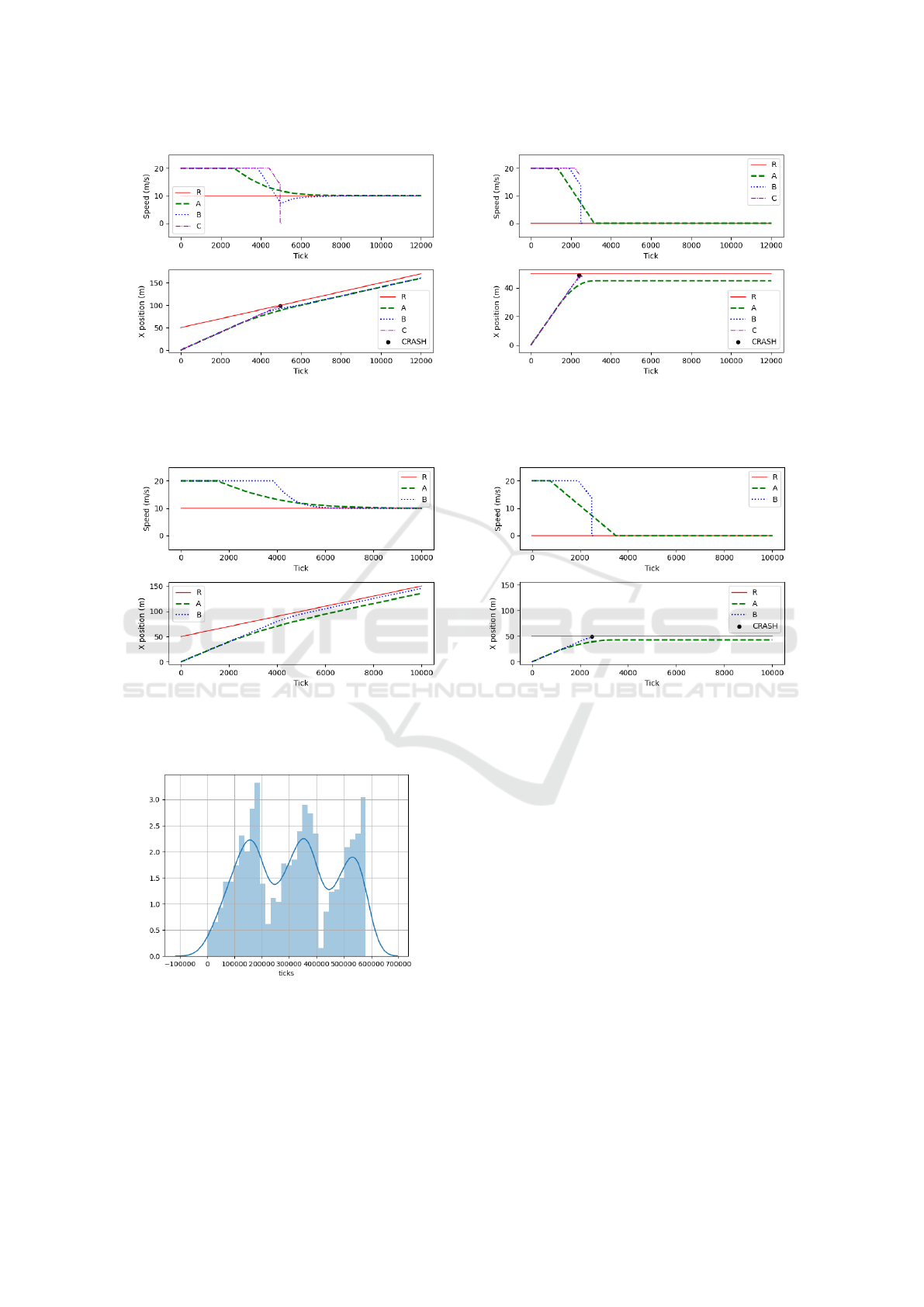
Figure 4a shows that A does not take risks: it per-
ceives far enough and thus starts braking in advance
to progressively adapt its speed to the slower pace of
the front vehicle. B has a shorter range of perception
and starts braking later. Its speed decreases abruptly,
down to 8m/s because the inter-vehicular distance to
the front-vehicle is not large enough. Once far enough
from R, it accelerates until it matches R’s speed. C
takes a lot of risk by driving at 20m/s while suffer-
ing from a small FFOV. It starts braking too late and
collides with R.
Figure 4b reproduces the same situation except
that R is immobile on the lane. A is still able to
stop safely, and C still collides with R after taking too
much risk. However, while B was safe before, it now
collides with R even if its behavior and setting do not
change. Indeed, an accident depends on the context.
In both cases, B does not drive according to its percep-
tion, but, during the first experiment, R was moving at
a slow pace, allowing B to stop soon enough to avoid
the collision. However, during the second experiment,
B brakes as soon as it perceives R, which is immobile,
but too late, and the collision is unavoidable.
Identical behaviors can either lead to a collision or
not, depending on the context. Facing a slow-driving
vehicle, it can avoid a collision even if it takes some
risks. However, the same vehicle driving according to
the same behavior will collide when facing an obsta-
cle, e.g., a broken-down vehicle.
4.3 Impact of k
2
: Inter-vehicle Distance
The environment required to illustrate the impact of
the inter-vehicle distance is similar to the one used to
demonstrate the impact of the FFOV, depicted in Fig-
ure 3. In these simulations, all vehicles have sufficient
perception even to stop facing an obstacle. However,
vehicles control the desired inter-vehicular distance,
according to k
2
. Shortening this distance may rep-
resent reasonable behavior under the assumption that
nothing unexpected arises (like the preceding vehicle
not braking too abruptly). The simulation settings are
identical to the ones described in Subsection 4.2. In-
deed, all simulations start with a reference vehicle R
driving at 10m/s only while the studied vehicle drives
at 20m/s. Different behavioral settings are compared:
A is a cautious vehicle k
2
A
= 1.0. B is a little riskier
k
2
B
= 0.5), whereas C is significantly riskier because
the inter-vehicular distance it is willing to allow with
the preceding vehicle is only a quarter of its stopping-
distance: k
2
C
= 0.25.
Figure 5a shows that a cautious vehicle like A does
not collide facing a broken-down vehicle or a slow-
moving one. C, which takes a lot of risks, crashes in
both cases. Even if its perception is sufficient, such a
vehicle does not react unless the inter-vehicular dis-
tance is insufficient to its liking. B, which is taking
some risks, may or may not collide according to the
context. If the preceding vehicle brakes too abruptly
(e.g., colliding itself with its front-vehicle), B col-
lides as illustrated in Figure 5b. Such behavior is
commonly observed on a highway with dense traffic.
Usually, no vehicle strictly complies with the safety
distance imposed by regulation, but most maintain a
reasonable inter-vehicular distance, allowing them to
brake safely. However, as soon as one collides, its
braking becomes unusual, and the next vehicle may
crash if they take too much risk.
4.4 Within a Traffic Flow
To evaluate the risk-taking parameters within a flow
of vehicles, we use generators that create an aver-
age vehicle number over a predefined period of ticks.
For instance, Figure 6 represents the number of vehi-
cles generated by periods of 2000 ticks. The gener-
ator uses the same generation rules and cycles three
times. Such a generator can generate any traffic den-
sity (even real-data describing flows).
We use such generators (one per lane) in a two-
lane environment to simulate congestion. However,
since all vehicles take few risks (from neutral to a risk
profile where k
i
= 0.75,∀i ∈ {0..4}). They adapt their
speed in due time, and eventually, all vehicles drive at
the same speed without colliding. Even if the initial
speeds of vehicles are different, they quickly converge
towards the same value.
However, as soon as 10% of vehicles generated
are willing to take more risks (down to a risk profile
k = (0.5, 0.5, 0.5, 0.5, 0.5)), collisions occur. A lot of
acceleration and braking (that mostly occurs when ve-
hicles change from one lane to another). Uncaring
vehicles do not consider the safety distance between
themselves and the one in the other lane. A chain of
braking interactions occurs and ends as soon as one
in the chain takes a little more risk than others and
crashes.
The environment considered is a two-lane high-
way 3 kilometers long where the speed limit is at
35m/s. A vehicle generator is placed at the beginning
Risk-oriented Behavior Design for Traffic Simulation
319
(a) R driving at 10m/s (b) R immobile
Figure 4: Speed and position of vehicles A, B and C (all driving at 20m/s) on the environment described Figure 3, facing a
vehicle R (a) driving at 10m/s or (b) immobile, according to different k
1
values.
(a) R driving at 10m/s (b) R immobile
Figure 5: Speed and position of vehicles A, B and C on the environment described Figure 3, facing a vehicle R (a) driving at
10m/s or (b) immobile, according to different k
2
values.
Figure 6: Number of vehicles generated per 2000 ticks-
period, cycling three times.
of each lane to certify the traffic density on the road.
These generators produce new vehicles regularly (ev-
ery 250 ticks), which do not take risks with k =
(1.1,1.1,1.1,1.1,1.1). At tick 10000, an important
increase in the generation rhythm, including uncaring
vehicles, characterized by k = (0.5,0.5,0.5,0.5,0.5)
during 10000 ticks. As depicted by Figure 7, it is
possible to evaluate the rate of vehicles crashing and
identify their type. Accidents occur as soon as the
proportion of uncaring vehicles in the environment
increases. Indeed, the actions of a few of them are
”swallowed” by the flow and others compensate for
the mistakes of these few. However, even if the gen-
eration of uncaring vehicles stops after 10000 ticks,
collisions continue to occur afterward. These vehi-
cles generate waves of braking that persist even after
they have passed.
5 CONCLUSION
Behavioral testing is becoming increasingly impor-
tant, especially with the interest in autonomous ve-
hicles. However, it is a difficult task as it requires
ICAART 2022 - 14th International Conference on Agents and Artificial Intelligence
320

Figure 7: Number of vehicles within different status in time.
subjecting the behavior to a significant but realistic
environmental stress to see how it reacts. Most of
the existing tools have different objectives and do not
focus on behavioral hypothesis testing, to study their
impact on road traffic.
The model we propose allows easy behavioral hy-
pothesis testing to generate realistic traffic whose be-
havior is individually configurable. This realistic traf-
fic is a complex system that can lead to the emergence
of accidents (unplanned, non-random). We argue that
risk-taking is an essential criterion to be taken into
account, but existing models are often based on phys-
ical phenomena, and their modification to integrate
these new aspects is not accessible to non-specialists.
The risk-taking profile is specific to each agent, so it
is possible to create flows of vehicles with heteroge-
neous behavior that take more or less risk. The risk
profile is based on five parameters and can be further
extended.
We show that, thanks to the proposed model, it
is possible to exhibit classic stylized facts in driv-
ing simulation and to study the behavioral factors that
lead to accidents. After the description of the model,
the simulation results clearly show classical phenom-
ena as well as unpredictable accidents due to interac-
tions between agents and their consequences on the
traffic.
REFERENCES
Al-Zinati, M. and Wenkstern, R. (2015). Matisse 2.0: A
large-scale multi-agent simulation system for agent-
based its. IAT’ 15, pages 328–335.
Ben-Akiva, M., Koutsopoulos, H., Toledo, T., Yang, Q.,
Choudhury, C., Antoniou, C., and Balakrishna, R.
(2010). Traffic simulation with mitsimlab. In Fun-
damentals of traffic simulation, pages 233–268.
Bonhomme, A., Mathieu, P., and Picault, S. (2016). A ver-
satile multi-agent traffic simulator framework based
on real data. IJAIT, 25(1):20.
Champion, A., Mandiau, R., Kolski, C., Heidet, A., and
Kemeny, A. (1999). Traffic generation with the
SCANeR™ simulator: towards a multi-agent architec-
ture. In DSC, pages 311–324.
Fellendorf, M. (1994). Vissim: A microscopic simulation
tool to evaluate actuated signal control including bus
priority. In 64th ITEAM, pages 1–9.
Gipps, P. G. (1981). A behavioural car-following model for
computer simulation. Transportation Research Part
B: Methodological, 15(2):105–111.
Iversen, H. (2004). Risk-taking attitudes and risky driving
behaviour. Transportation Research Part F: Traffic
Psychology and Behaviour, 7(3):135–150.
Kesting, A., Treiber, M., and Helbing, D. (2007). General
lane-changing model mobil for car-following models.
Transportation Research Board, 1(1999):86–94.
Krajzewicz, D., Bonert, M., and Wagner, P. (2006).
The open source traffic simulation package sumo.
RoboCup 2006.
Krauß, S. (1998). Microscopic modeling of traffic flow: In-
vestigation of collision free vehicle dynamics. PhD
thesis, Dt. Zentrum f
¨
ur Luft-und Raumfahrt eV, Abt.
Unternehmensorganisation und . . . .
Ram, T. and Chand, K. (2016). Effect of drivers’ risk per-
ception and perception of driving tasks on road safety
attitude. Transportation Research Part F: Traffic Psy-
chology and Behaviour, 42:162–176.
Tlig, M., Buffet, O., and Simonin, O. (2012). Coopera-
tive behaviors for the self-regulation of autonomous
vehicles in space sharing conflicts. In ICTAI, pages
1126–1132.
Treiber, M., Hennecke, A., and Helbing, D. (2000). Con-
gested traffic states in empirical observations and mi-
croscopic simulations. Physical review E, 62(2):1805.
Treiber, M. and Kesting, A. (2010). An open-source micro-
scopic traffic simulator. IEEE ITSM, 2(3):6–13.
Wegener, A., Pi
´
orkowski, M., Raya, M., Hellbr
¨
uck, H.,
Fischer, S., and Hubaux, J.-P. (2008). Traci: An in-
terface for coupling road traffic and network simula-
tors. In Proceedings of the 11th Communications and
Networking Simulation Symposium, CNS ’08, page
155–163, New York, NY, USA. Association for Com-
puting Machinery.
Risk-oriented Behavior Design for Traffic Simulation
321
