
Look before You Leap! Designing a Human-centered AI System for
Change Risk Assessment
Binay Gupta, Anirban Chatterjee, Subhadip Paul, Matha Harika, Lalitdutt Parsai,
Kunal Banerjee
a
and Vijay Agneeswaran
Walmart Global Tech, Bangalore, Karnataka, India
binay.gupta, anirban.chatterjee, subhadip.paul0, matha.harika, lalitdutt.parsai,
Keywords:
Change Management, Human-centerd AI, Explainable AI, Concept Drift.
Abstract:
Reducing the number of failures in a production system is one of the most challenging problems in tech-
nology driven industries, such as, the online retail industry. To address this challenge, change management
has emerged as a promising sub-field in operations that manages and reviews the changes to be deployed in
production in a systematic manner. However, it is practically impossible to manually review a large number
of changes on a daily basis and assess the risk associated with these. This warrants the development of an
automated system to assess the risk associated with a large number of changes. There are a few commercial
solutions available to address this problem but those solutions lack the ability to incorporate domain knowl-
edge and continuous feedback from domain experts into the risk assessment process. As part of this work, we
aim to bridge the gap between model-driven risk assessment of change requests and the assessment of domain
experts by building a continuous feedback loop into the risk assessment process. Here we present our work to
build an end-to-end machine learning system along with the discussion of some of the practical challenges we
faced related to extreme skewness in class distribution, concept drift, estimation of the uncertainty associated
with the model’s prediction and the overall scalability of the system.
1 INTRODUCTION
In any technology driven industry, launch of a new
business or launch of new product features for an ex-
isting business to customers requires a series of soft-
ware changes to a base system that is already in pro-
duction. Each of these changes carries with it some
likelihood of failure. Reducing the number of fail-
ures in a production system is one of the key chal-
lenges. It is especially important in the current era of
agile development that has a tight delivery schedule.
The situation may be further exacerbated when there
is a large volume of changes, which severely restricts
thorough inspection and review before deployment.
From our experience, another impediment in man-
ual change risk assessment occurs when the risk for
a change is marked as “low” by the change requester
(which, in reality, need not be so – this may happen
if the developer is new or less skilled, and hence has
applied poor judgement); such requests are often ig-
nored altogether by domain experts while reviewing,
a
https://orcid.org/0000-0002-0605-630X
and these may manifest as critical issues later in the
pipeline. In fact, in the context of Walmart, we ob-
serve that a substantial percentage
1
of major produc-
tion issues occur due to planned and so-called “low-
risk” changes in e-commerce market and US stores.
The monetary impact of these major issues is also
quite significant
1
. The number of such changes per
week is so high
1
on average that it is practically im-
possible to manually review all these change requests
due to limited bandwidth of the human experts. This
necessitated the development of an automated risk as-
sessment system for change requests.
In this paper, we present our experience of explor-
ing the following questions while building an auto-
mated risk assessment system:
• Can we reliably build a failure probability model
for changes which can provide actionable insights
from the change data to the change management
team?
1
We abstain from providing the exact numbers to main-
tain confidentiality.
Gupta, B., Chatterjee, A., Paul, S., Harika, M., Parsai, L., Banerjee, K. and Agneeswaran, V.
Look before You Leap! Designing a Human-centered AI System for Change Risk Assessment.
DOI: 10.5220/0010877500003116
In Proceedings of the 14th International Conference on Agents and Artificial Intelligence (ICAART 2022) - Volume 3, pages 655-662
ISBN: 978-989-758-547-0; ISSN: 2184-433X
Copyright
c
2022 by SCITEPRESS – Science and Technology Publications, Lda. All rights reserved
655

• Can we optimally seek feedback from the domain
experts for the model’s inference on a limited
number of changes so that it improves the model’s
performance as well as does not over-burden the
domain experts with feedback requests?
The remainder of this paper is organized as fol-
lows. In Section 2, we provide an overview of the
problem. In Section 3, we provide a brief descrip-
tion of our dataset. In Sections 4 & 5, we elaborate
on the end-to-end system and its deployment, respec-
tively. Section 6 sheds light on explainability tech-
niques utilized by us for user adoption. In Sections 7
& 8, we talk about the business impact of this solution
and some of the interesting observations we made in
the course of this work, respectively, and finally, we
conclude this paper in Section 9.
2 PROBLEM OVERVIEW
Our main goal is to determine if we can predict the
probability that a change will cause a major produc-
tion issue based on the information available for that
change request. Prediction at an earlier stage is likely
to be much less precise, and prediction at a later
stage would be much less useful because fewer op-
tions would be available to mediate the risk.
2.1 Inherent Challenges
One of the major problems that we have faced is im-
balance in the class distribution of the data. It makes
machine learning model bias towards predicting ma-
jority class, which in turn leads to high false negative
rate and monetary loss. Also, during holiday period
(October–December), the number of change requests
drops sharply because associates avoid pushing risky
changes in the production. This creates cyclical shift
in the data distribution. Additionally, process changes
in operation, formation or merger of teams lead to
gradual concept drifts. Along with these difficulties,
running the system in production seamlessly on large
amounts of data makes the problem even more chal-
lenging.
3 DATA DESCRIPTION
We have collected change request data for one year.
Each instance in this data consists of several attributes
or features. We can logically divide these into four
primary categories:
• Descriptive Feature: These are plain text infor-
mation about the change, such as, change sum-
mary, change description, and a few others.
• Q & A Feature: These are the answers provided
by the change requester to a set of predefined
questions, such as, “whether the change was pre-
viously implemented or not”, etc.
• Team Profile: This information is not readily
available with the change data but we derive it
from the historical data. These features primar-
ily reflect the tendency of a team to raise change
requests which create major issues in production.
• Change Importance: These features reflect the
perception of the change requester regarding the
impact, importance and the risk of a change re-
quest.
We also associate labels with every change data
instance. We associate the changes, which did not
create any major production issue, with the label “nor-
mal”. We label the others as “risky”. Our train-
ing sample consists of 600K change instances among
which only 540 belong to the class “risky”, which is
only 0.09% of all the change instances.
4 RISK ASSESSMENT SYSTEM
We build an automated risk assessment system which
has conceptually three main functional components:
• data collection and preparation,
• model training and monitoring,
• model inferencing and gathering of expert’s feed-
back.
Figure 1 illustrates a conceptual diagram of our end-
to-end system workflow. We explain all the functional
components of the system in the following subsec-
tions.
4.1 Data Collection and Preparation
In this part of the system, we collect change related
data from multiple sources and aggregate these. Once
aggregated, we prepare the training data for the sub-
sequent training stage. It is important to mention here
that we pose this task as a classification problem with
a high degree of class imbalance. A subset of fea-
tures that we use for training the classification model
are raw attributes of the change requests, and such
change attributes are readily available in change data
that we collect. However, some of the features that
ICAART 2022 - 14th International Conference on Agents and Artificial Intelligence
656
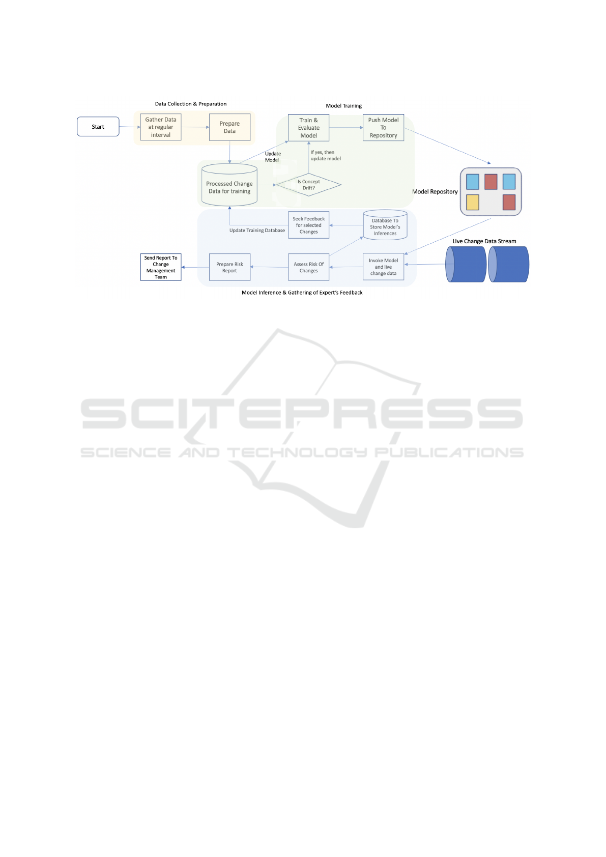
Figure 1: Conceptual diagram of end-to-end system workflow.
we feed to the machine learning (ML) model are de-
rived features, such as, the features to indicate the de-
gree of severity expressed in the change description
or a team’s tendency to cause major production issues
through changes, and many others.
Next, during processing phase we impute miss-
ing values, encode categorical features, up-sample in-
stances from minority class to generate the final train-
ing data. Linear regression is applied to impute miss-
ing values. Both label encoding and one-hot encoding
are used for categorical features judiciously. Brute
force up-sampling of minority class can cause over-
fitting. Similarly, we may end up discarding poten-
tially useful information if we randomly downsample
instances from the majority class. To mitigate both
the problems, we have used GAMO (Mullick et al.,
2019), where only safe samples from minority class
are used to synthesis new instances, thus we can avoid
generating noisy and boundary samples. More details
on different up-sampling strategies is given in Sec-
tion 8.
4.2 Model Training and Monitoring
We use a gradient-boosted decision tree (XG-
Boost) (Chen and Guestrin, 2016) to generate the
probability with which a new change request may
cause major issues in production, and this ML model
is at the core of this system. We consider this proba-
bility as the estimation of the risk for a change.
Note that during model training phase, we have
tried both supervised and unsupervised models be-
fore deciding on which algorithm will perform best.
One-class support vector machine and isolation forest
are the two algorithms we have explored from unsu-
pervised classification paradigm. Among supervised
learning algorithms, we have analyzed performance
of logistic regression, XGBoost and Deep Neural Net-
works (DNNs). Unsupervised ML algorithms are use-
ful in absence of class labels; however, these meth-
ods always under-performed compared to supervised
learning methods. Logistic regression assumes lin-
ear relationship between dependent and independent
variable, which may not always hold true, as in our
case. Gradient boosting and DNNs emerge as clear
winners as they can learn complex functions better.
As XGBoost is less resource intensive and explaining
a model’s decision is easier in this case, we have de-
cided to go with XGBoost. While choosing best set
of hyper-parameters, we have used Bayesian hyper-
parameter optimization technique (Wu et al., 2019).
We will provide a comparative analysis of these mod-
els subsequently in Section 7.
4.2.1 Concept Drift
We generally train the model once in a month. How-
ever, we have a system in place to monitor any sig-
nificant shift in data pattern which may substantially
degrade the performance of the model (see Figure 1).
In case we detect any such drift, we initiate an out-
of-cycle training of the model with the latest change
data. This kind of drift in data pattern is called con-
cept drift and is formally defined as follows:
∃X : p
t0
(X, y) 6= p
t1
(X, y) (1)
This definition explains concept drift as the change
in the joint probability distribution for input X and
prediction y between two time points t0 and t1.
Look before You Leap! Designing a Human-centered AI System for Change Risk Assessment
657

4.2.2 Detection of Concept Drift
We use a modified form of Kolmogorov-Smirnov (KS)
Test to detect concept drift in data. Before we intro-
duce how we apply it in this context, we first briefly
review the standard form of KS Test.
Suppose we have two samples A and B containing
univariate observations. We would like to know with a
significance level of α, whether we can reject the null
hypothesis that the observations in A and B originate
from the same probability distribution. If no informa-
tion is available regarding the data distribution, it is
safe to assume that the drawn observations are i.i.d.,
we can use the rank-based KS test to verify the pro-
posed hypothesis. According to it, we can reject the
null hypothesis at level α if the following inequality
is satisfied:
D > c(α)
r
n + m
nm
(2)
where the value of c(α) can be retrieved from a known
table, n is the number of observations in A and m is
the number of observations in B. The right side of the
inequality is the target p-value. D is the Kolmogorov-
Smirnov statistic, i.e., the obtained p-value, and is de-
fined as follows:
D = sup
x
|F
A
(x) − F
B
(x)| (3)
where
F
A
(x) =
1
|A|
∑
a∈A,a≤x
1, F
B
(x) =
1
|B|
∑
b∈B,b≤x
1 (4)
F(·) represents cumulative distribution function. We
note that D can actually be computed as follows:
D = max
x∈A∪B
|F
A
(x) − F
B
(x)| (5)
In order to quantify drift we use a modified version
of KS algorithm. We first measure the drift in each
and every feature and later we combine them using
weighted average. More formally, we compute the
final drift between two multi-variate samples of data
as follows:
D
f inal
=
1
K
K
∑
i=1
w
i
D
i
(6)
where D
i
is the measured drift in i
th
feature between
the two samples according to KS algorithm and w
i
is
the importance of i
th
feature as computed by XGBoost
while training and K is the total number of features.
Once the value of D
f inal
crosses a certain thresh-
old, it raises an alarm to update the model by re-
training. While training the model, we assign higher
weights to more recent data points so that the model
is more tuned to the latest pattern in the dataset.
4.3 Model Inferencing and Gathering of
Expert’s Feedback
This part of the system is responsible for ingesting the
live change data in batches into the system, running
the latest version of the model against these to gener-
ate the risk scores and sending back the risk report to
the change management team.
It is also responsible for gathering expert’s
feedback on a small sample of changes. It seeks an
expert’s feedback only for those changes for which
the model exhibited a high degree of uncertainty.
It actually ranks all the change requests in a batch
according to their estimated uncertainty of prediction
and sends top m change requests to experts for feed-
back. The subsection below provides a brief overview
of how we estimate the predictive uncertainty of the
model.
Estimation of Predictive Uncertainty. While
predictive uncertainty is widely studied for deep
learning based models (Lai et al., 2021; Gal, 2016),
the topic seems to be under-explored for gradient
boosting based models, such as, XGBoost. We esti-
mate the uncertainty associated with the predictions
of the model within standard Bayesian ensemble
based framework (Gal, 2016).
In a general setting of supervised learning by an en-
semble of models, we can approximate the predictive
posterior of the ensemble as follows by using the
posterior probability p(θ|D) of the ensemble, where
θ and D represent the model parameters and training
data respectively.
P(y|x, D) = E
p(θ|D)
[P(y|x;θ)]
≈
1
M
M
∑
m=1
P(y|x;θ
(m)
)
(7)
In above equation, θ
(m)
∼ p(θ|D) and y represents
the prediction of the model while M represents the
number of models in the ensemble. The entropy es-
timated for the predictive posterior i.e. P(y|x, D) of
a model represents the total uncertainty of the model.
Total uncertainty is contributed by both data uncer-
tainty and knowledge uncertainty. Conceptually, we
express the uncertainty associated with a prediction of
the model as the mutual information between model
parameters θ and prediction y. We can estimate the
mutual information between model parameters θ and
prediction y as given below (Andrey Malinin and Us-
ICAART 2022 - 14th International Conference on Agents and Artificial Intelligence
658

timenko, 2021):
I [y, θ|x, D] = H [P(y|x, D)] − E
p(θ|D)
[H [P(y|x, θ)]]
≈ H [
1
M
M
∑
m=1
P(y|x;θ
(m)
)]
−
1
M
M
∑
m=1
H [P(y|x; θ
(m)
)]
(8)
Here, x represents the feature-set corresponding
to the prediction y, D = {x
(i)
, y
(i)
}
N
i=1
represents the
entire dataset and M is the total number of trees con-
structed by XGBoost. This is expressed as the differ-
ence between the entropy (H ) of the predictive poste-
rior, a measure of total uncertainty, and the expected
entropy of each model in the ensemble, a measure of
expected data uncertainty. Their difference is a mea-
sure of ensemble diversity and estimates knowledge
uncertainty.
5 DEPLOYMENT AND
MONITORING
We deploy the entire system as a workflow on an in-
ternal machine learning platform. Currently, it pro-
cesses around 60K change requests per week. We
have a dashboard in place to monitor several met-
rics related to the business impact of the system. The
dashboard gets updated as soon as new data comes
in. We build the pipeline for drift detection and the
subsequent retraining of the model, as required, using
MLFlow (Zaharia et al., 2018).
6 EXPLAINABILITY FOR USER
ADOPTION
Adding explainability to the predictions made by an
AI system is often a crucial pre-requisite for its adop-
tion, especially, if the users are not well-versed in
AI, and hence may be apprehensive of using the so-
lution (Gade et al., 2019; David et al., 2021). Con-
sequently, we explored some interpretable ML tech-
niques, including both global explanations and local
explanations, to augment our predictions with suit-
able explanations. For global explanation, we tried
the surrogate model approach (Molnar et al., 2020),
where a simpler (easy to explain) model is trained
to approximate the predictions of a larger complex
model. We chose the decision tree as the surrogate
model because decision trees are, arguably, the easi-
est to interpret, and hence for our (uninitiated to AI)
users, decision tree was the best stepping stone into
explainable AI. Figure 2 shows an example of a deci-
sion tree used as a surrogate model for global expla-
nation when trained on a subset of 341 samples; we
refrain from showing the final decision tree trained on
all the samples for confidentiality reasons – however,
note that the example shown here is similar to the fi-
nal one. In this example, the root node corresponds
to the variable which tries to capture how risky is the
change request according to the requester. In case the
request is regarded as risky, then the next node checks
whether the change count, i.e., the number of change
requests raised by a change request team over a pe-
riod of one year, is less than 187 or not - note that
the value 187 is determined automatically based on
Gini impurity of a node split (Leo Breiman, 1984);
on the other hand, if the request is not deemed to be
risky, then the next thing to consider is whether the
requester belongs to a particular group or not. For
each node, the number of samples that belongs to its
left and right child is provided as #obs, and for the
leaf nodes, their Gini Impurity is mentioned. It may
be noted that for our final decision tree, which we
obtained through extensive experimentation including
tuning several hyper-parameters, had its predictions
matched with that of the deployed XGBoost model in
∼ 70% cases – although a higher number would have
indicated that the surrogate model mimics the origi-
nal one more closely, it is not unexpected that there
will be considerable difference in accuracies between
two ML models with different learning capabilities.
Moreover, we found that the global surrogate model
gives satisfactory explanations for most of the cases
involving risky change requests, which our users are
more interested in.
For local explanations, we use Local Interpretable
Model-agnostic Explanations (LIME) (Ribeiro et al.,
2016). To explain an individual prediction, LIME
method perturbs the original input to create a set of
new inputs and records their corresponding outputs.
It then tries to fit a linear regression model to this set
of inputs and outputs, weighed by the distance of each
input to the original one – the basic assumption being
that even if a model is overall non-linear, in a small
bounded region it behaves linearly. This linear model
is finally used to explain the original prediction. Fig-
ure 3 shows an example of a LIME plot that is de-
clared to be risky; note that all the features in this ex-
ample indicate that the request is risky except for one
“complexity of implementation” – cumulatively, the
decision taken is risky. It may be interesting to note
that SHapley Additive exPlanations (SHAP) (Lund-
berg and Lee, 2017) is another popular method used
in explaining ML models that gives both global and
Look before You Leap! Designing a Human-centered AI System for Change Risk Assessment
659
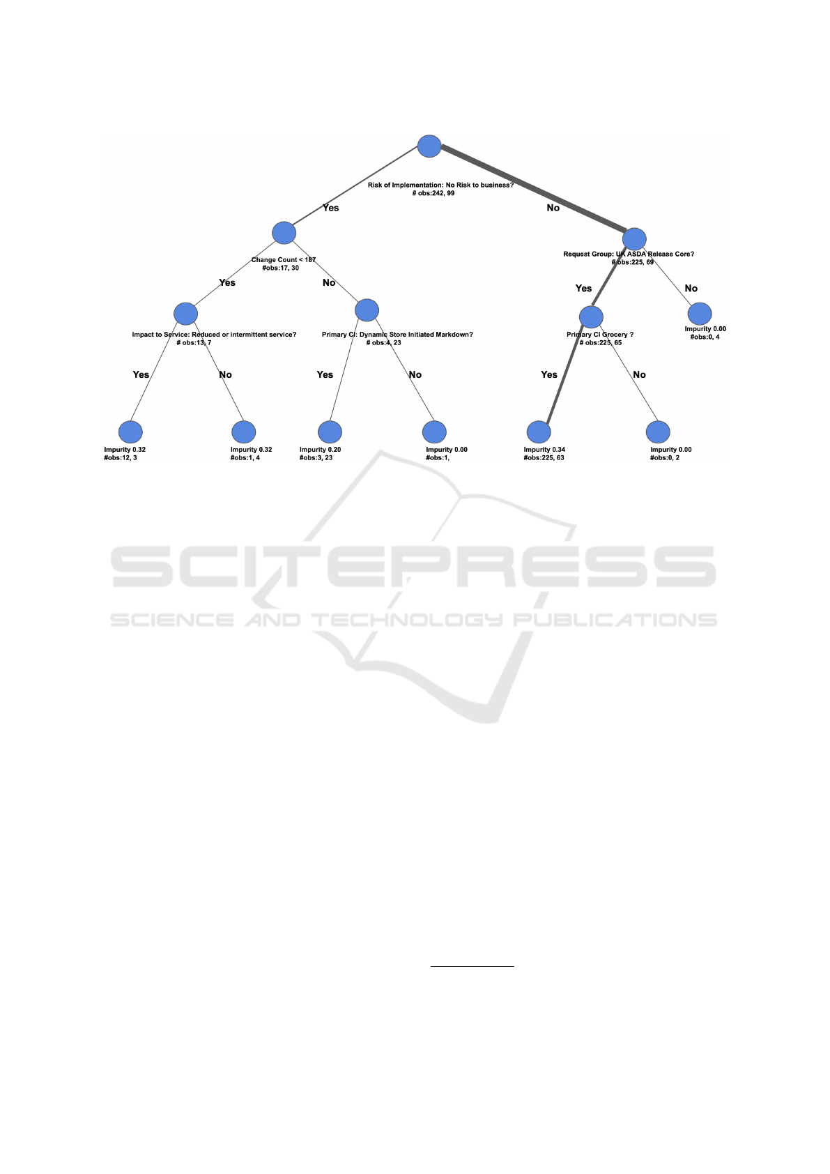
Figure 2: An example of a decision tree used as a surrogate model for global explanation of change request risk assessment.
local explanations; however, we found that our users
preferred the decision tree and LIME over SHAP for
explanations, and hence we subsequently exclude it in
our deployment.
7 MODEL PERFORMANCE AND
BUSINESS IMPACT
7.1 Model’s Performance
We explore multiple options such as one-class SVM,
isolation forest, logistic regression, deep neural net-
work and XGBoost, to identify change requests with
high risk. We consider true positive rate (TPR) and
false positive rate (FPR) as the performance met-
rics for the models. As Table 1 suggests, deep neu-
ral network and XGBoost exhibit much better per-
formance than the other methods we explored. To
choose between XGBoost and deep neural network,
we compute the positive likelihood ratio and XG-
Boost emerges the winner with respect to this metric.
We computed all these metrics to evaluate a model’s
performance against a validation dataset.
7.2 Business Impact
We primarily monitor two metrics to keep track of
the business impact: number of major issues per
10000 CRQ (change requests) and percentage of man-
machine agreement.
Figure 4 represents the month-over-month (MoM)
improvement in the number of major issues per 10000
CRQ from January, 2021 to July, 2021. We observe
around 85% decline in this metric in July, 2021 with
respect to January, 2021
2
. We attribute the slight in-
crease in this metric in June with respect to May to
concept drift in data but we could reverse this trend
by proactive detection of concept drift and subsequent
retraining of the model.
Percentage of man-machine agreement is a metric
which represents the percentage of high risk changes
as predicted by the model, which have actually been
accepted as the high risk changes by domain experts.
It is primarily an indicative of the confidence of busi-
ness on this predictive system. Figure 5 represents
month-over-month improvement in this metric from
January, 2021 to July, 2021
2
. Observe a slight dip in
this metric in March and June with respect to Febru-
ary and May respectively. However, this trend has
never lasted because of the continuous gathering of
feedback from domain experts and incorporating the
same into the model.
Post deployment, the production team has con-
firmed that the number of major incidents has been
reduced by 33% with net savings ranging into multi-
million dollars as in Q2 of 2021. Note that there may
be other factors (e.g., software design changes) that
have contributed to the savings; however, it is ac-
knowledged that our AI based prediction system has
2
We provide the relative variations of this metric MoM.
Absolute values of this metric are confidential.
ICAART 2022 - 14th International Conference on Agents and Artificial Intelligence
660
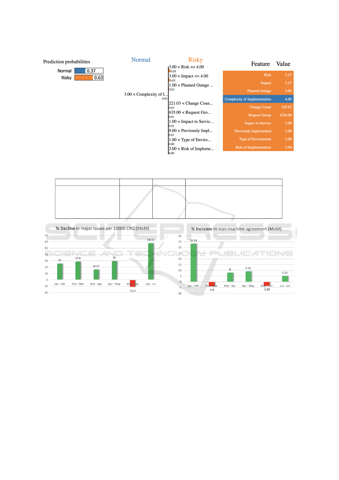
Figure 3: An example of a LIME plot used for local explanation of a change request risk assessment.
Table 1: Comparative Analysis of ML Algorithms.
Algorithm TPR(%) FPR(%) Positive Likelihood Ratio (TPR/FPR)
One Class SVM 52.7 ± 0.01 18.6 ± 0.01 2.83
Isolation Forest 51.3 ± 0.03 18.9 ± 0.03 2.71
Logistic Regression (LR) 62.5 ± 0.01 14.5 ± 0.01 4.31
Deep Neural Network 79.1 ± 0.02 9.7 ± 0.02 8.15
XGBoost 78.9 ± 0.01 9.1 ± 0.01 8.67
Figure 4: Percentage decline in major production issues
(CRQ = change requests, MoM = month-over-month).
definitely played a key role. From prior records of the
benefits that these software changes typically brought,
their contribution in the recent savings should be in
the ballpark of 30%, while the rest 70% may be at-
tributed to our new machine learning based risk as-
sessment system.
8 SOME OBSERVATIONS
We share some of the interesting observations we
made while building this system and how we dealt
with these.
Figure 5: Percentage improvement in man-machine agree-
ment (CRQ = change requests, MoM = month-over-month).
8.1 Up-sampling Minority Class
We observed a significant variablity (see Table 2)
in model’s performance with different up-sampling
methods. Since using GAMO (Mullick et al., 2019)
resulted in maximum benefit, we decided to use it.
8.2 Data Sparsity & Imputation Method
Missing values are very common among most of the
tabular datasets like ours. There are many methods
available to impute the missing values in a dataset.
However, if the degree of sparsity is high and the
missing values are not imputed with high accuracy,
Look before You Leap! Designing a Human-centered AI System for Change Risk Assessment
661

Table 2: Experiments With Different Up-sampling Techniques in Learning By Oversampling.
XGBoost with Different Up-sampling Methods TPR(%) FPR(%)
XGBoost + SMOTE (Bunkhumpornpat et al., 2009) 77.1 ± 0.01 10.4 ± 0.01
XGBoost + AdaSyn-SMOTE (Gameng et al., 2019) 77.0 ± 0.01 10.6 ± 0.01
XGBoost + cGAN (Douzas and Bac¸
˜
ao, 2017) 78.5 ± 0.01 9.4 ± 0.01
XGBoost + DOS (Ando and Huang, 2017) 78.6 ± 0.01 9.3 ± 0.01
XGBoost + GAMO (Mullick et al., 2019) 78.9 ± 0.01 9.1 ± 0.01
it takes a toll on the generalization error of the model.
An intuitive reason behind this is the fact that inaccu-
rate imputation of data with high degree of sparsity,
significantly alters the distribution of the data after
imputation. It eventually results in the model learn-
ing a distribution which is significantly different from
the ground-truth of the distribution. We observed
that complex model-based imputation methods, such
as MINWAE (Mattei and Frellsen, 2019), yield bet-
ter true and false positive rate from the same model
in comparison to simple mean or median imputation
methods.
9 CONCLUSION
In this paper, we introduce a human-centered AI
based change risk assessment system which aims to
bridge the gap between model-based assessment of
change risks and the assessment by the domain ex-
perts. While designing the system, we faced many
challenges, such as, extreme class imbalance, gradual
concept drifts, model selection, explaining the predic-
tions for user adoption, scaling at an industrial level.
We also elaborate on how this system created business
impact post deployment. In near future, we will ex-
plore an active-learning based framework to leverage
the experts’ feedback more effectively.
REFERENCES
Ando, S. and Huang, C. (2017). Deep over-sampling
framework for classifying imbalanced data. In ECML
PKDD, volume 10534 of Lecture Notes in Computer
Science, pages 770–785. Springer.
Andrey Malinin, L. P. and Ustimenko, A. (2021). Uncer-
tainty in gradient boosting via ensembles. In ICLR.
Bunkhumpornpat, C., Sinapiromsaran, K., and Lursinsap,
C. (2009). Safe-level-SMOTE: Safe-level-synthetic
minority over-sampling technique for handling the
class imbalance problem. In Advances in Knowledge
Discovery and Data Mining, pages 475–482.
Chen, T. and Guestrin, C. (2016). XGBoost: A scalable tree
boosting system. In KDD, pages 785–794.
David, D. B., Resheff, Y. S., and Tron, T. (2021). Explain-
able AI and adoption of financial algorithmic advi-
sors: An experimental study. In AIES, pages 390–400.
Douzas, G. and Bac¸
˜
ao, F. (2017). Effective data generation
for imbalanced learning using conditional generative
adversarial networks. Expert Systems with Applica-
tions, 91.
Gade, K., Geyik, S. C., Kenthapadi, K., Mithal, V., and Taly,
A. (2019). Explainable AI in industry. In KDD, pages
3203–3204.
Gal, Y. (2016). Uncertainty in Deep Learning. PhD thesis,
University of Cambridge.
Gameng, H. A., Gerardo, B. B., and Medina, R. P. (2019).
Modified adaptive synthetic SMOTE to improve clas-
sification performance in imbalanced datasets. In IC-
ETAS, pages 1–5.
Lai, Y., Shi, Y., Han, Y., Shao, Y., Qi, M., and Li, B. (2021).
Exploring uncertainty in deep learning for construc-
tion of prediction intervals. CoRR, abs/2104.12953.
Leo Breiman, Jerome Friedman, C. J. S. R. O. (1984).
Classification and Regression Trees. Chapman and
Hall/CRC.
Lundberg, S. M. and Lee, S. (2017). A unified approach
to interpreting model predictions. In NeurIPS, pages
4765–4774.
Mattei, P.-A. and Frellsen, J. (2019). MIWAE: Deep gen-
erative modelling and imputation of incomplete data
sets. In ICML, volume 97 of Proceedings of Machine
Learning Research, pages 4413–4423. PMLR.
Molnar, C., Casalicchio, G., and Bischl, B. (2020). Inter-
pretable machine learning - A brief history, state-of-
the-art and challenges. In ECML PKDD, volume 1323
of Communications in Computer and Information Sci-
ence, pages 417–431.
Mullick, S. S., Datta, S., and Das, S. (2019). Generative
adversarial minority oversampling. In ICCV, pages
1695–1704.
Ribeiro, M. T., Singh, S., and Guestrin, C. (2016). ”Why
should I trust you?”: Explaining the predictions of any
classifier. In KDD, pages 1135–1144.
Wu, J., Chen, X.-Y., Zhang, H., Xiong, L.-D., Lei, H., and
Deng, S.-H. (2019). Hyperparameter optimization for
machine learning models based on Bayesian optimiza-
tion. Journal of Electronic Science and Technology,
17(1):26–40.
Zaharia, M., Chen, A., Davidson, A., Ghodsi, A., Hong,
S. A., Konwinski, A., Murching, S., Nykodym, T.,
Ogilvie, P., Parkhe, M., Xie, F., and Zumar, C.
(2018). Accelerating the machine learning lifecycle
with mlflow. IEEE Data Eng. Bull., 41(4):39–45.
ICAART 2022 - 14th International Conference on Agents and Artificial Intelligence
662
