Automatic Label Detection in Chest Radiography Images

ao Pedrosa

1,2 a

, Guilherme Aresta

1,2 b

, Carlos Ferreira

1,2 c

Ana Maria Mendonc¸a

1,2 d

and Aur

elio Campilho

1,2 e

Institute for Systems and Computer Engineering, Technology and Science (INESC TEC), Porto, Portugal

Faculty of Engineering of the University of Porto (FEUP), Porto, Portugal

Keywords:

Chest Radiography, Deep Learning, Object Detection, Classiﬁcation Bias, Markers.

Abstract:

Chest radiography is one of the most ubiquitous medical imaging exams used for the diagnosis and follow-up

of a wide array of pathologies. However, chest radiography analysis is time consuming and often challeng-

ing, even for experts. This has led to the development of numerous automatic solutions for multipathology

detection in chest radiography, particularly after the advent of deep learning. However, the black-box nature

of deep learning solutions together with the inherent class imbalance of medical imaging problems often leads

to weak generalization capabilities, with models learning features based on spurious correlations such as the

aspect and position of laterality, patient position, equipment and hospital markers. In this study, an automatic

method based on a YOLOv3 framework was thus developed for the detection of markers and written labels

in chest radiography images. It is shown that this model successfully detects a large proportion of markers

in chest radiography, even in datasets different from the training source, with a low rate of false positives per

image. As such, this method could be used for performing automatic obscuration of markers in large datasets,

so that more generic and meaningful features can be learned, thus improving classiﬁcation performance and

robustness.

1 INTRODUCTION

Chest radiography (CXR), also known as chest x-ray,

is one of the most ubiquitous medical imaging ex-

ams and remains extremely advantageous thanks to

its wide availability, low cost, portability and low ra-

diation dosage in comparison to other ionizing imag-

ing modalities. Moreover, radiologists typically use

CXRs for the diagnosis or screening of multiple con-

ditions associated to the chest wall and the lungs as

well as the heart and greater vessels. Nevertheless,

the assessment of CXR images is time consuming and

often challenging, even for experts. Furthermore, the

large quantity of CXR exams acquired per day can

lead to an unmanageable workload for radiologists,

leading to misdiagnosis.

As such, computer-aided diagnosis (CAD) sys-

tems for CXR pathology detection have long been

proposed, providing a valuable 2

opinion for radi-

https://orcid.org/0000-0002-7588-8927

https://orcid.org/0000-0002-4856-138X

https://orcid.org/0000-0001-6754-6495

https://orcid.org/0000-0002-4319-738X

https://orcid.org/0000-0002-5317-6275

ologists or screening abnormal cases that radiologists

should assess visually. Traditional machine learning

approaches have mostly been applied for the detection

of a speciﬁc disease (Qin et al., 2018), speciﬁcally,

for lung nodule and tuberculosis detection. However,

these algorithms fail to represent the wide array of

pathologies encountered in the clinical environment.

The recent advent of deep learning, as well as the

release of large CXR datasets such as ChestXRay-8

(Wang et al., 2017) and CheXpert (Irvin et al., 2019),

have fostered the development of multi-disease detec-

tion approaches, while simultaneously improving per-

formance in the detection of single pathologies (Irvin

et al., 2019).

However, the intrinsic nature of deep learning

techniques, where image features are learned from an

image-level label (normal vs pathological or pathol-

ogy A vs B) can lead to unexpected behaviour and

low explainability. In fact, in complex images such

as CXR and in severe imbalance of classes and data,

there is no guarantee that the decisions made by a

deep learning system are representative of a clinical

ﬁnding and not a spurious correlation of the data. In-

deed, recent algorithms for COVID-19 detection in

Pedrosa, J., Aresta, G., Ferreira, C., Mendonça, A. and Campilho, A.

Automatic Label Detection in Chest Radiography Images.

DOI: 10.5220/0010888100003123

In Proceedings of the 15th International Joint Conference on Biomedical Engineering Systems and Technologies (BIOSTEC 2022) - Volume 2: BIOIMAGING, pages 63-69

ISBN: 978-989-758-552-4; ISSN: 2184-4305

CXR were shown to have learned correlations in the

data rather than clinical information (DeGrave et al.,

2020). Because most models for COVID-19 detec-

tion are trained with a mixture of negative COVID-19

pre-pandemic CXRs and positive COVID-19 cases, it

becomes simpler to learn shortcuts such as the dataset

from where the image comes from than more complex

features such as lung opacities. While these shortcuts

lead to excellent performance in datasets similar to

the train dataset, catastrophic failure occurs once the

model is tested on a different dataset. Among others,

the markers for laterality, patient positioning and hos-

pital system were identiﬁed as features strongly in-

ﬂuencing the decision of algorithms (DeGrave et al.,

2020).

The goal of this study was thus to develop and

validate an automatic method to detect markers and

written labels in CXR images. Such a method could

then be used for automatic obscuration of markers in

large datasets, promoting the learning of generic and

meaningful features and thus improving performance

and robustness.

2 METHODS

2.1 Datasets

Four different datasets were used in this study,

obtained from different sources. The ﬁrst dataset,

hereinafter referred to as the Mixed dataset (1,395

CXRs) is composed of a combination of multiple pub-

lic CXR datasets, namely from the CheXpert (Irvin

et al., 2019) (7 CXRs), ChestXRay-8 (Wang et al.,

2017) (226 CXRs), Radiological Society of North

America Pneumonia Detection Challenge (RSNA-

PDC) (Kaggle, 2018) (639 CXRs) and COVID

DATA SAVE LIVES

(199 CXRs) datasets as

well as from COVID-19 CXR public repositories,

namely COVID-19 IDC (Cohen et al., 2020) (265

CXRs), COVIDx (Wang and Wong, 2020) (4 CXRs),

Twitter

(9 CXRs) and the Sociedad Espa

nola de

Radiologia M

edica (SERAM) website

(46 CXRs).

The second and third datasets, hereinafter referred

to as the BIMCV and COVIGR datasets (289 and

300 CXRs respectively) are each from a single

hospital system public dataset, namely the BIMCV-

COVID19-PADCHEST (Bustos et al., 2020) (248

https://www.hmhospitales.com/coronavirus/

covid-data-save-lives

https://twitter.com/ChestImaging

https://seram.es/images/site/TUTORIAL CSI RX

TORAX COVID-19 vs 4.0.pdf

CXRs) and BIMCV-COVID-19+ (Vay

a et al., 2020)

(41 CXRs) datasets and the COVIDGR (Tabik et al.,

2020) dataset. The fourth dataset is a private col-

lection of 597 CXRs collected retrospectively at the

Centro Hospitalar de Vila Nova de Gaia e Espinho

(CHVNGE) in Vila Nova de Gaia, Portugal between

the 21st of March and the 22nd of July of 2020. All

data was acquired under approval of the CHVNGE

Ethical Committee and was anonymized prior to any

analysis to remove personal information.

All CXRs were selected randomly from both nor-

mal and pathological cases after exclusion of views

other than postero-anterior and antero-posterior.

2.2 CXR Annotation

In order to set a ground truth for training and evalu-

ation of the algorithms, manual annotation of all la-

bels was performed using an in-house software. The

software presented CXRs from a randomly selected

subset and allowed for window center/width adjust-

ment, zooming and panning. The software allowed

for rectangles of any size to be drawn on the image,

covering the labels, and saved the corresponding co-

ordinates. Figure 1 shows examples of manually an-

notated bounding boxes.

2.3 Automatic Label Detection

The automatic label detection model is based on

YOLOv3 (You Only Look Once, Version 3) (Red-

mon and Farhadi, 2018). The network is composed

of a feature extraction backbone, DarkNet-53 (Red-

mon and Farhadi, 2018), which is used to obtain

a M ×M ×N feature map F, where M is the spa-

tial grid used and N is the number of feature maps.

This feature map F is then convolved to obtain an

M×M×B×6 output tensor where B is a predeﬁned

number of objects to predict per grid point and which

contains the predicted objects’ conﬁdence score, class

probability and bounding box position and dimen-

sions. One particular characteristic of YOLOv3 is that

the bounding box dimensions are not explicitly pre-

dicted by the network but are deﬁned in relation to

pre-deﬁned bounding box templates, commonly re-

ferred to as anchors. The anchors are learned a pri-

ori before the training of YOLOv3 and correspond

to the cluster centers from a k-means that maximizes

the IoU of these anchors with the training set ground

bounding boxes. The network then learns to predict

the deviation (in length and width) from each of these

pre-deﬁned anchors, thus deﬁning each predicted ob-

ject.

BIOIMAGING 2022 - 9th International Conference on Bioimaging

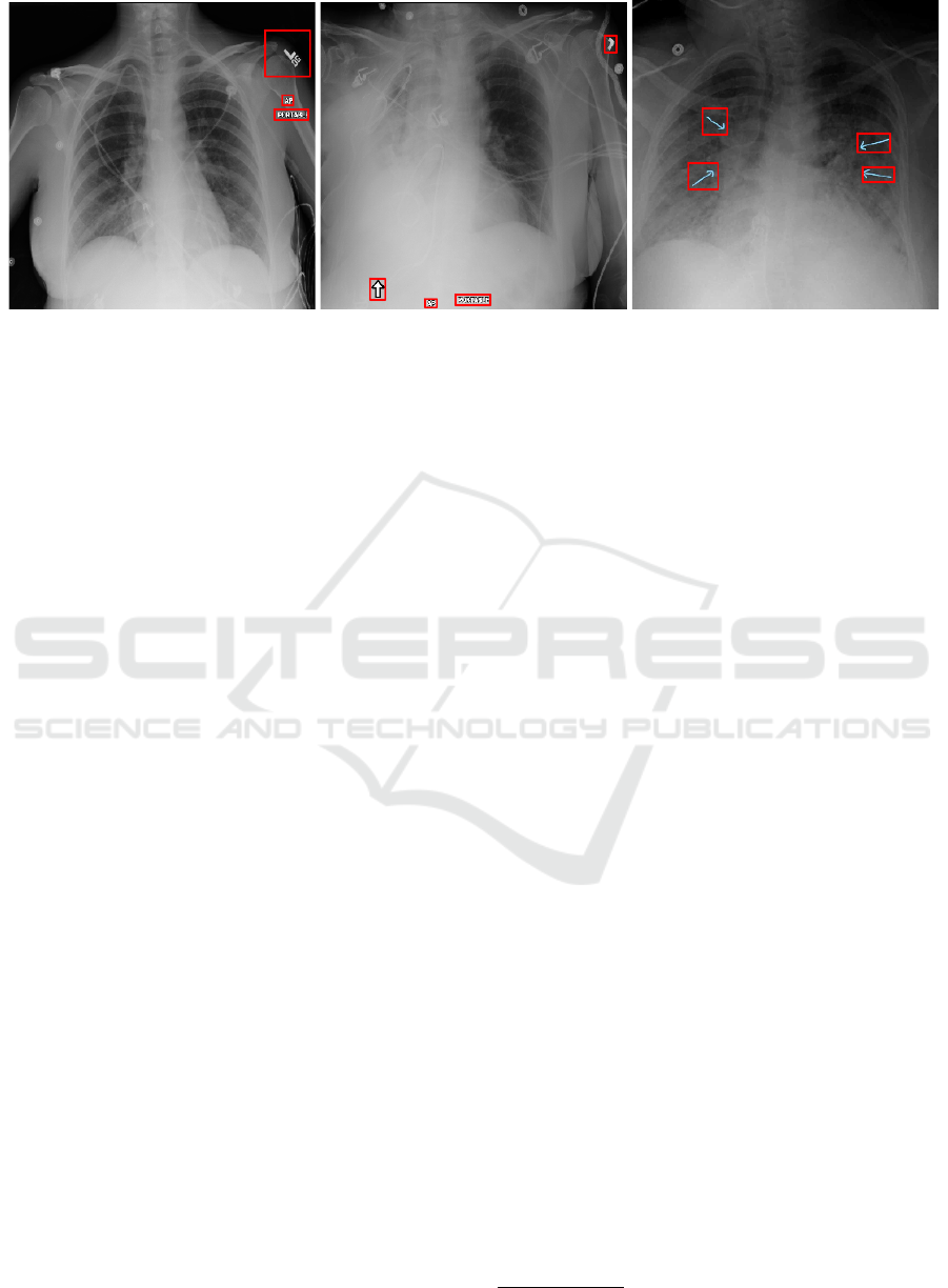
Figure 1: Example CXRs from the Mixed dataset with annotated bounding boxes covering equipment, laterality and patient

position markers among others.

In practice, this means that YOLOv3 divides the

image into a grid, deﬁned according to M, and pre-

dicts objects for each image patch. For each object, a

conﬁdence score and class probability are predicted,

as well as position and dimensions in relation to the

most similar anchor. During inference, predicted ob-

jects with low conﬁdence score are then discarded to

obtain the ﬁnal prediction.

3 EXPERIMENTS

3.1 CXR Annotation

Manual annotation was performed for all CXRs, re-

sulting in 1,202, 210, 656 and 1,298 annotated bound-

ing boxes for the Mixed, BIMCV, COVIDGR and

CHVNGE datasets respectively, which correspond to

an average of 1.51 bounding boxes per CXR.

3.2 Model Training

One quarter of the Mixed dataset was used for train-

ing/validation, ensuring that the same patient did not

appear in both training and testing. In total, 317 CXRs

(643 bounding boxes) were used for training and 39

CXRs (77 bounding boxes) were used for valida-

tion. The feature extraction backbone is the DarkNet-

53 (Redmon and Farhadi, 2018), and each cell has as-

sociated 9 anchor boxes. YOLOv3 pretrained weights

on MS-COCO (Lin et al., 2014) were used for initial-

ization. Training is performed with a batch size of 2,

Adam optimizer (Kingma and Ba, 2014) and learn-

ing rate of 10

−4

. The learning rate was lowered by

a factor of 10 whenever the validation loss did not

improve for 2 epochs and training was stopped if the

loss did not improve for 7 epochs. Data augmentation

was performed by applying random translations, ﬂips

and scale changes. All experiments were conducted

on an Intel Core i7-5960X@3.00GHz, 32GB RAM,

2×GTX1080 desktop using Python 3.6, Tensorﬂow

2.0.0 and Keras 2.3.1.

3.3 Model Evaluation

Model evaluation was performed in terms of sensitiv-

ity and false positives (FP) per CXR. In a ﬁrst ex-

periment, model predictions were compared to the

ground truth manual annotations for the Mixed test

set and the remaining datasets (BIMCV, COVIDGR

and CHVNGE). A prediction was considered a true

positive if it matches a ground truth bounding box.

Given that ground truth labels were obtained through

manual annotation and do not represent the minimum

bounding box for each label, a prediction was consid-

ered to be a match to a ground truth label if a coverage

of 40% was achieved.

In order to perform a more extensive validation

of the model, a subset of 100 CXRs was randomly

selected from all datasets and labels were then arti-

ﬁcially placed in each CXR. Two additional experi-

ments were then conducted considering: 1) random

individual letters and 2) random English words

. For

each experiment, a total of 4,032 artiﬁcial labels were

placed per CXR, resulting in 403,200 artiﬁcially la-

beled CXRs per experiment. CXRs were divided into

8×8 quadrants and an equal number of labels was ran-

domly placed within each quadrant. Different label

font heights and intensity values were also consid-

ered, speciﬁcally font heights of 1/2, 1/4, 1/8, 1/16,

1/32, 1/64 and 1/128 in relation to CXR height and

relative intensity values of 0, 1/4, 1/2, 3/4, 1, 5/4, 3/2,

7/4 and 2. Label intensity values > 1 correspond to

artiﬁcial labels with intensity higher than the origi-

nal maximum image intensity. All parameters were

https://www.mit.edu/$\sim$ecprice/wordlist.10000

Automatic Label Detection in Chest Radiography Images

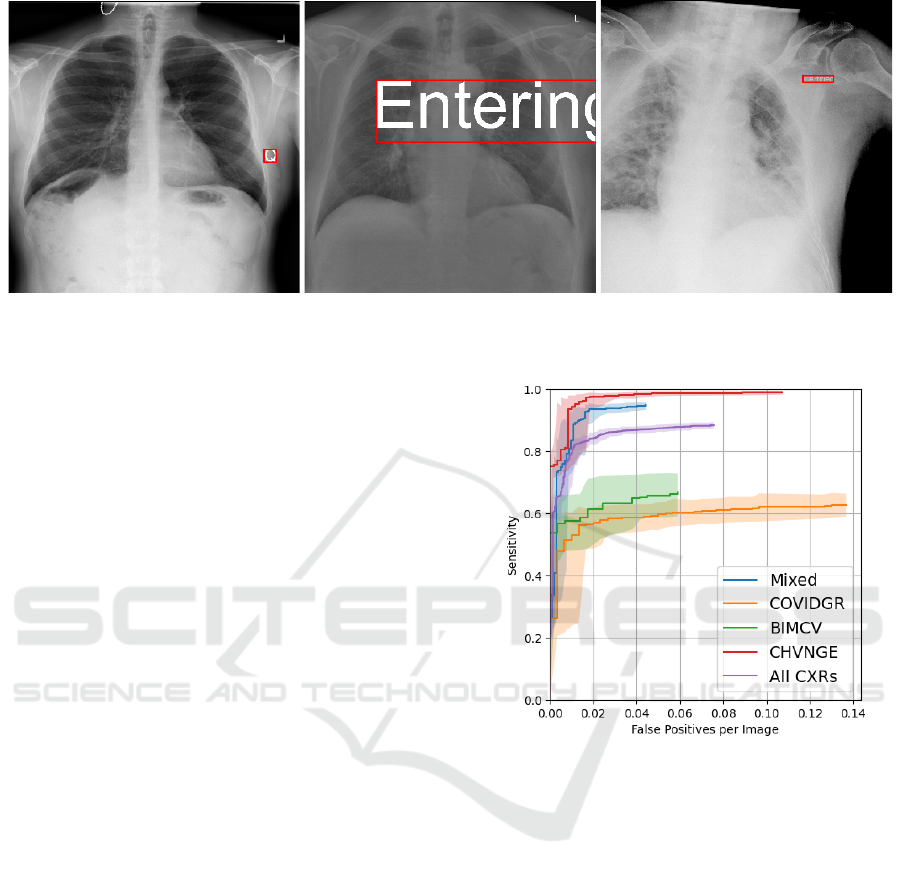
Figure 2: Example CXRs with artiﬁcially generated labels and corresponding minimum bounding boxes. (left) Label “Q” with

brightness 2 and font height 1/16; (middle) Label “Entering” with brightness 1.5 and font height 1/4; (right) Label “Certiﬁed”

with brightness 0.75 and font height 1/32.

selected empirically for an adequate representation

of label variability and sensitivity analysis. Figure 2

shows examples of artiﬁcially generated labels. Given

the goal of label obscuration, label coverage was also

used for evaluation for these experiments, deﬁned as

the percentage of the area of the reference bounding

box covered by the predicted bounding box.

For all experiments, statistical error estimation

was performed by computing the 95% bias corrected

and accelerated (BC

) bootstrapping conﬁdence in-

terval (CI) (Efron, 1987) calculated with 5.000 iter-

ations.

4 RESULTS

Figure 3 shows the free-response operating character-

istic (FROC) curve obtained for the ground truth la-

bels for all images and for each dataset, excluding the

CXRs used for training. It can be seen that a high

sensitivity is obtained for the Mixed and CHVNGE

datasets, while sensitivity for the COVIDGR and

BIMCV datasets saturates at approximately 0.6. All

datasets exhibit low FP rate per CXR. Figure 4 shows

examples of CXRs with ground truth and predicted

bounding boxes.

Figure 5 shows the sensitivity and coverage of the

artiﬁcial labels as a function of font height, relative

brightness and label position. Relative brightness was

computed as the difference between the artiﬁcial label

intensity and the average intensity of the CXR within

the minimum bounding box of the label.

Figure 3: FROC curve on all CXRs and each dataset.

Shaded region corresponds to the 95% BC

CI of each

FROC curve.

5 DISCUSSION

Figure 3 shows that a low number of FPs was

obtained, with high sensitivity, particularly for the

Mixed and CHVNGE datasets, in spite of the rela-

tively small training set used. As shown in Figure

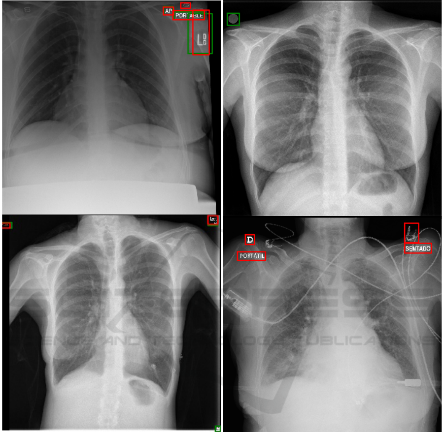
4, the model was able to successfully distinguish be-

tween elements that belong to the original CXR and

those that were placed later. However, as illustrated

by the lower sensitivity obtained for COVIDGR and

BIMCV, the model struggled with faint and radio-

logical laterality markers (Fig. 4(b)) and particularly

small equipment markers (Fig. 4(c)) which were not

present in the training set.

Figure 5 further highlights the model capabilities,

showing that good sensitivity and coverage can be

obtained for both bright and dark labels, at differ-

BIOIMAGING 2022 - 9th International Conference on Bioimaging

(a) (b)

Figure 4: Example CXRs showing ground truth (green) and predicted (red) bounding boxes. (a) Mixed CXR; (b) BIMCV

CXR showing missed laterality marker; (c) COVIGR CXR showing missed equipment marker (right lower corner); (d)

CHVNGE CXR showing FP (medical device).

ent font sizes. As expected, subtle labels with rela-

tive brightness close to zero are more difﬁcult to de-

tect, as well as extremely smalls labels at font sizes

under 1/32. Total label coverage is obtained for al-

most all font sizes, outside the more subtle relative

brightness ranges. Naturally, for extremely large font

sizes (over 1/8), coverage signiﬁcantly drops as the

model struggles to identify words/letters as single la-

bels and instead predicts independent sections of the

label, thus failing to cover the signiﬁcant portion of

CXR that falls within the label minimum bounding

box (Fig. 2 center). Surprisingly, slightly higher sen-

sitivity was observed for letters/words with negative

relative brightness for smaller objects (font height be-

low 1/8), which correspond to objects darker than the

background. Given that most of the ground truth an-

notations are of positive relative brightness, it can be

expected that the YOLOv3 has learnt to detect strong

edges, independent of the signal of the relative bright-

ness of the objects, which can be seen as proof of the

robustness of this method. Regarding the position of

the label, it can be seen that labels in the upper corners

can be detected more successfully, as most CXR la-

bels are placed in those regions, but reasonable perfor-

Automatic Label Detection in Chest Radiography Images

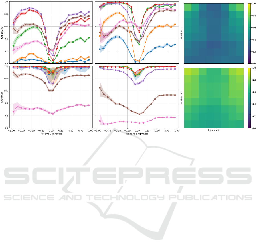
Figure 5: Sensitivity and coverage as a function of font height and relative brightness on the artiﬁcial letter (left) and word

(center) labels and sensitivity as a function of CXR position on the artiﬁcial letter (top right) and word (bottom right) labels.

Plot colors correspond to font height: • - 1/128; • - 1/64; • - 1/32; • - 1/16; • - 1/8; • - 1/4; • - 1/2. Shaded region

corresponds to the 95% BC

CI of each curve.

mance is nonetheless obtained in the remaining CXR

regions.

In spite of the promising results obtained, there are

limitations to this study which should be addressed.

A more thorough cross-dataset validation could be

performed and training with both manually annotated

and artiﬁcially generated labels could yield beneﬁts

by improving performance for subtle and small labels

and for the lower portion of the CXR. Nevertheless,

in light of the low number of FPs per CXR and as

previously suggested, this framework could be used

to automatically obscurate markers in large datasets

with minimum oversight, potentially improving the

learning of generic and meaningful features. Alterna-

tively, it could also be used retrospectively in trained

models to infer whether shortcuts related to markers

have been learned by the model by computing the fre-

quency with which a model highlights image markers

as responsible for a given decision. Both these tech-

niques will be approached in future work.

6 CONCLUSION

In conclusion, an automatic CXR label detection

framework was proposed in this study based on a

YOLOv3 architecture. In spite of the relatively small

training set, it was shown that the model can be suc-

cessfully applied to datasets other than the training

data and good performance was shown for differ-

ent font sizes, relative brightness and position, being

thus an efﬁcient method for label obscuration in large

datasets, potentially improving robustness and gener-

alization.

ACKNOWLEDGEMENTS

The authors would like to thank the Centro Hos-

pitalar de Vila Nova de Gaia/Espinho, Vila Nova

de Gaia (CHVNGE), Portugal for making the data

available which made this study possible. This

work was funded by the ERDF - European Regional

Development Fund, through the Programa Opera-

cional Regional do Norte (NORTE 2020) and by Na-

tional Funds through the FCT - Portuguese Foun-

dation for Science and Technology, I.P. within the

scope of the CMU Portugal Program (NORTE-01-

0247-FEDER-045905) and UIDB/50014/2020. Guil-

herme Aresta and Carlos Ferreira are funded by

the FCT grant contracts SFRH/BD/120435/2016 and

SFRH/BD/146437/2019 respectively

BIOIMAGING 2022 - 9th International Conference on Bioimaging

REFERENCES

Bustos, A., Pertusa, A., Salinas, J.-M., and de la Iglesia-

Vay

a, M. (2020). Padchest: A large chest x-ray image

dataset with multi-label annotated reports. Medical

Image Analysis, 66:101797.

Cohen, J. P., Morrison, P., and Dao, L. (2020). Covid-19 im-

age data collection. arXiv preprint arXiv:2003.11597.

DeGrave, A. J., Janizek, J. D., and Lee, S.-I. (2020). AI

for radiographic COVID-19 detection selects short-

cuts over signal. medRxiv.

Efron, B. (1987). Better bootstrap conﬁdence inter-

vals. Journal of the American statistical Association,

82(397):171–185.

Irvin, J., Rajpurkar, P., Ko, M., Yu, Y., Ciurea-Ilcus, S.,

Chute, C., Marklund, H., Haghgoo, B., Ball, R., Sh-

panskaya, K., et al. (2019). CheXpert: A large chest

radiograph dataset with uncertainty labels and expert

comparison. In Proceedings of the AAAI Conference

on Artiﬁcial Intelligence, volume 33, pages 590–597.

Kaggle (2018). RSNA pneumonia detection chal-

lenge — kaggle. https://www.kaggle.com/c/

rsna-pneumonia-detection-challenge/. (Accessed on

10/07/2020).

Kingma, D. P. and Ba, J. (2014). Adam: A

method for stochastic optimization. arXiv preprint

arXiv:1412.6980.

Lin, T.-Y., Maire, M., Belongie, S., Hays, J., Perona, P.,

Ramanan, D., Doll

ar, P., and Zitnick, C. L. (2014).

Microsoft coco: Common objects in context. In Euro-

pean conference on computer vision, pages 740–755.

Springer.

Qin, C., Yao, D., Shi, Y., and Song, Z. (2018). Computer-

aided detection in chest radiography based on artiﬁcial

intelligence: a survey. Biomedical engineering online,

17(1):113.

Redmon, J. and Farhadi, A. (2018). Yolov3: An incremental

improvement. arXiv preprint arXiv:1804.02767.

Tabik, S., G

omez-R

ıos, A., Mart

ın-Rodr

ıguez, J.,

Sevillano-Garc

ıa, I., Rey-Area, M., Charte, D.,

Guirado, E., Su

arez, J., Luengo, J., Valero-

Gonz

alez, M., et al. (2020). COVIDGR dataset and

COVID-SDNet methodology for predicting COVID-

19 based on chest x-ray images. arXiv preprint

arXiv:2006.01409.

Vay

a, M. d. l. I., Saborit, J. M., Montell, J. A., Pertusa,

A., Bustos, A., Cazorla, M., Galant, J., Barber, X.,

Orozco-Beltr

an, D., Garcia, F., et al. (2020). BIMCV

COVID-19+: a large annotated dataset of RX and

CT images from COVID-19 patients. arXiv preprint

arXiv:2006.01174.

Wang, L. and Wong, A. (2020). COVID-Net: A tailored

deep convolutional neural network design for detec-

tion of COVID-19 cases from chest x-ray images.

arXiv preprint arXiv:2003.09871.

Wang, X., Peng, Y., Lu, L., Lu, Z., Bagheri, M., and

Summers, R. M. (2017). Chestx-ray8: Hospital-

scale chest x-ray database and benchmarks on weakly-

supervised classiﬁcation and localization of common

thorax diseases. In Proceedings of the IEEE Con-

ference on Computer Vision and Pattern Recognition,

pages 2097–2106.

Automatic Label Detection in Chest Radiography Images