
On the Choice of General Purpose Classifiers in Learned Bloom Filters:
An Initial Analysis Within Basic Filters
Giacomo Fumagalli
1 a
, Davide Raimondi
1 b
, Raffaele Giancarlo
2 c
, Dario Malchiodi
1,3 d
and Marco Frasca
1,3 e
1
Dipartimento di Informatica, Universit
`
a degli Studi di Milano, 20133 Milan, Italy
2
Dipartimento di Matematica ed Informatica, Universit
`
a di Palermo, 90133 Palermo, Italy
3
CINI National Laboratory in Artificial Intelligence and Intelligent Systems (AIIS), Universit
`
a di Roma, 00185 Roma, Italy
Keywords:
Learned Bloom Filters, Learned Data Structures, Information Retrieval, Classification.
Abstract:
Bloom Filters are a fundamental and pervasive data structure. Within the growing area of Learned Data
Structures, several Learned versions of Bloom Filters have been considered, yielding advantages over classic
Filters. Each of them uses a classifier, which is the Learned part of the data structure. Although it has a central
role in those new filters, and its space footprint as well as classification time may affect the performance of
the Learned Filter, no systematic study of which specific classifier to use in which circumstances is available.
We report progress in this area here, providing also initial guidelines on which classifier to choose among five
classic classification paradigms.
1 INTRODUCTION
Learned Data Structures is a novel area at the cross-
road of Classic Data Structures and Machine Learn-
ing. They have been initially proposed by Kraska et.
al. (Kraska et al., 2018) and have had a rapid growth
(Ferragina and Vinciguerra, 2020a). Moreover, now
the area has been extended to include also Learned
Algorithms (Mitzenmacher and Vassilvitskii, 2020).
The theme common to those new approaches to Data
Structures Design and Engineering is that a query to a
data structure is either intermixed with or preceded by
a query to a Classifier (Duda et al., 2000) or a Regres-
sion Model (Freedman, 2005), those two being the
learned part of the data structure. To date, Learned In-
dexes have been the most studied, e.g., (Amato et al.,
2021; Ferragina and Vinciguerra, 2020b; Ferragina
et al., 2021; Kipf et al., 2020; Kraska et al., 2018;
Maltry and Dittrich, 2021; Marcus et al., 2020a; Mar-
cus et al., 2020b). Rank/select data structures have
also received some attention (Boffa et al., 2021).
a
https://orcid.org/0000-0002-2068-9293
b
https://orcid.org/0000-0001-8171-8302
c
https://orcid.org/0000-0002-6286-8871
d
https://orcid.org/0000-0002-7574-697X
e
https://orcid.org/0000-0002-4170-0922
Bloom Filters (Bloom, 1970), which are the object
of this study, have also been considered, as we detail
next. Historically, they have been designed to be a
data structure able to solve the Approximate Mem-
bership Problem in small space (see Section 2). Due
to their fundamental nature and pervasive use, many
variants and alternatives have been proposed. A good
review in the domain of Internet applications is pro-
vided in (Broder and Mitzenmacher, 2002).
Kraska et al. (Kraska et al., 2018) have proposed
a learned version of such a filter, in which a query to
the data structure is preceded by a query to a suit-
ably trained binary classifier. The intent is to re-
duce space and reject time. Mitzenmacher (Mitzen-
macher, 2018) has provided a model for those filters,
together with a very informative mathematical anal-
ysis of their pros/cons and even an alternative pro-
posal. Additional Learned Bloom Filters have been
proposed recently (Dai and Shrivastava, 2020; Vaidya
et al., 2021). It is worth pointing out that, although
they differ in architecture, each of those proposals has
a classifier as its central part.
Somewhat puzzling is that, although the classifier
is the novel part of this new family of Filters and it
is accounted for in theoretical studies (Mitzenmacher,
2018), not much attention is given to which classifier
Fumagalli, G., Raimondi, D., Giancarlo, R., Malchiodi, D. and Frasca, M.
On the Choice of General Purpose Classifiers in Learned Bloom Filters: An Initial Analysis Within Basic Filters.
DOI: 10.5220/0010889000003122
In Proceedings of the 11th International Conference on Pattern Recognition Applications and Methods (ICPRAM 2022), pages 675-682
ISBN: 978-989-758-549-4; ISSN: 2184-4313
Copyright
c
2022 by SCITEPRESS – Science and Technology Publications, Lda. All rights reserved
675

to use in practical settings. Kraska et al. use a Neu-
ral Network, while Dai and Shrivastava and Vaidya et
al. use Random Forests. Those choices are only in-
formally motivated, giving no evidence of superiority
with respect to other possible ones, via a comparative
analysis. Therefore, the important problem of how to
choose a specific classifier in conjunction with a spe-
cific filter has not been addressed so far, even in one
application domain.
Such a State of the Art is problematic, both
methodologically and practically. Here we propose
the first, although initial, study that considers the
choice of the classifier within Learned Filters. Since
our study is of a fundamental nature, we consider only
basic versions of the Filters and six generic, if not
textbook, classifier paradigms. The intent is to char-
acterize how different classifiers affect different per-
formance parameters of the Learned Filter. The ap-
plication domain is the one of malicious URL deter-
mination, as in previous work. As per literature stan-
dard, our datasets are real and fall within the data size
used by Dai and Shrivastava. However, even so, Ran-
dom Forest classifiers do not seem to be competitive
in our setting, needing bigger datasets. Indeed, for the
continuation of this work, we plan to consider much
larger datasets and include also Random Forests. Ad-
ditional application domains will also be considered.
Our results provide a confirmation of some ex-
pected behaviours, like that more complex classifiers
tend to yield larger space reduction when used within
a learned Bloom Filter, but also some counterintuitive
perspectives, including that simple linear classifiers
might represent very competitive alternatives to their
bigger counterparts, sometimes even better. These re-
sults make more sense if we consider that in a learned
Bloom Filter classifiers come up with one or two clas-
sic Bloom Filters, calibrated in turn on the classifier
performance, and accordingly it is their synergy that
determines the overall space reduction, not just the
classifier itself. Finally, a relevant note is also that in
our experiments linear classifiers allow two orders of
magnitude faster reject times.
2 APPROXIMATE SET
MEMBERSHIP PROBLEM:
DEFINITIONS AND KEY
PARAMETERS
Definition. Given S ⊂ U and x ∈ U, where U is
the universe of keys, the set membership problem
consists in finding a data structure able to determine
if x ∈ S. The approximate set membership instead
allows for a fraction ε of false positives, that is
elements in U \ S considered as members of S. No
false negatives are allowed. That is, elements in S
considered as non-members.
A Paradigmatic Example. Assume that a set of
URLs is given. They can be malicious, i.e., websites
hosting unsolicited content (spam, phishing, drive-by
downloads, etc.), or luring unsuspecting users to be-
come victims of scams (monetary loss, theft of private
information, and malware installation), or otherwise
labeled as benign. The aim is to design a time ef-
ficient data structure that takes small space and that
“rejects” benign URL quickly, as they do not belong
to the malicious set. On occasions, we may have false
positives.
Key Parameters of the Filter. The reject time,
taken as the expected time to reject a non-member of
the set; the space taken by the data structure, since
the cardinality of S may be very large; the false pos-
itive rate ε. Quite remarkably, Bloom provided two
data structures to solve the posed problem, linking the
three key parameters in trade-off bounds. The most
space-efficient of those data structures goes under the
name of Bloom Filter and it is outlined next, together
with two of its learned versions.
2.1 Basic Classic and Learned Bloom
Filters
Classic. Letting |S| = n, a Bloom Filter (BF) is
made up by a bit array v of size m, whose elements
are all initialized to 0. It uses k hash functions
h
j
: U −→ {0, 1, . . . , m − 1}, j ∈ {1, . . . , k}, which
can be assumed to be perfect in theoretic studies (see
(Mitzenmacher, 2018)). When a new element x of S is
added, it is coded using the hash functions: each bit in
v in position h
j
(x) is set to 1, for each j ∈ {1, . . . , k}.
To test if a key x ∈ U is a member of S, h
j
(x) for each
j is computed, and x will be rejected if there exists
j ∈ {1, . . ., k} such that v[h
j
(x)] = 0. However, when
the Bloom Filter considers x as a member, it might
be a false positive due to the hash collisions. The
false positive rate ε is inversely related to the space
usage of the bit array. More accurately, the trade-off
formula connecting the key parameters of the Filter is
given in equation (21) in (Bloom, 1970). Analogous
trade-off formulas are also known, e.g., (Broder
and Mitzenmacher, 2002; Mitzenmacher, 2018). In
applications (Broder and Mitzenmacher, 2002), one
usually asks for the the most space-conscious filter,
ICPRAM 2022 - 11th International Conference on Pattern Recognition Applications and Methods
676

given a false positive rate, being the reject time
a consequence of those choices.
Learned: One Classifier and One Filter. The in-
tent of this data structure, named Learned Bloom Fil-
ter (LBF), is to achieve a given false positive rate, as
in a classic filter, but in less space, and possibly with
little loss in reject time (Kraska et al., 2018). One
can proceed as follows. A classifier C : U −→ [0, 1] is
trained on a labeled dataset (x, y
x
), where x ∈ D ⊂ U ,
S ⊂ D, and y
x
= 1 when x ∈ S, y
x
= −1 otherwise. The
positive class is thereby the class of keys S. The larger
C(x), the more likely x belongs to S. Then, in order
to have a binary prediction, a threshold τ ∈ (0, 1) is to
be fixed, yielding positive predictions for any x ∈ U
such that C(x) ≥ τ, negative otherwise. To avoid false
negatives in the learned Bloom Filter, that is elements
x ∈ S rejected by the filter, a classic “backup” Bloom
Filter F is created on the set {x ∈ S|C(x) < τ}. A
generic key x is tested against membership in S by
computing the corresponding prediction C(x): x is
considered as an element of S if C(x) ≥ τ or C(x) < τ
and F does not reject x. x is rejected otherwise. Un-
like a classic Bloom Filter, the false positive rate of
a LBF depends on the distribution of a given query
set
¯
S ∈ U \ S (Mitzenmacher, 2018). Hereafter, we
will refer to ε
τ
= |{x ∈
¯
S|(C(x) ≥ τ)}| as the empir-
ical false positive rate of the classifier on
¯
S, to ε
F
as
the false positive rate of F, and to the empirical false
positive rate of the LBF on
¯
S as ε = ε
τ
+ (1 − ε
τ
)ε
F
.
Fixed a desired ε, the optimal value of ε
F
is
ε
F
=
ε − ε
τ
1 − ε
τ
,
which yields the constraint ε
τ
< ε.
It is to be pointed out that now, false positive rate
ε, space and reject time of the entire filter are inti-
mately connected and influenced by the choice of τ.
Another delicate point that emerges from the analy-
sis offered in (Mitzenmacher, 2018) is that, while the
false positive rate of a classic Filter can be reliably
estimated experimentally because of its data indepen-
dence, for the Learned version this is no longer so
immediate and further insights are needed. As an ad-
ditional contribution, an experimental methodology is
suggested in (Mitzenmacher, 2018) and we adhere to
it here.
Learned: Sandwiched Classifier. The intent of
this variant, named Sandwiched Learned Bloom Filter
(SLBF), is to filter out most non-keys before they are
supplied to the LBF. This would allow the construc-
tion of a much smaller backup filter F and an overall
more compact data structure (Mitzenmacher, 2018).
The specifics follow. A Bloom Filter I for the set
S precedes the structure of the Learned Bloom Filter
described in the previous paragraph. The subsequent
LBF is constructed on the elements of S not rejected
by I. Clearly, I might yield a considerable number of
false positives, when a limited budget of bits is dedi-
cated to it. A query x ∈ U is rejected by the SLBF if I
rejects it, otherwise the results of the subsequent LBF
is returned. Denoted by ε
I
the false positive rate of
the filter I, the empirical false positive rate of a SLBF
is ε = ε
I
ε
τ
+ (1 − ε
τ
)ε
F
. For a desired value of ε,
the following properties hold (Mitzenmacher, 2018):
• ε
I
=
ε
ε
τ
1 −
FN
n
, with FN number of false nega-
tives of C;
• ε
1 −
FN
n
≤ ε
τ
≤ 1 −
FN
n
.
As for the previous learned Bloom Filter variant, the
classifier accuracy affects all the key factors of a
SLBF, namely false positive rate, space and reject
time. Considerations and experimental methodolo-
gies in this case are the same as in the previous case.
3 EXPERIMENTAL
METHODOLOGY
3.1 General Purpose Classifiers
The classifiers used in our analysis are briefly de-
scribed below. We assume each x ∈ U is repre-
sented through a set of n real-valued attributes A =
{A
1
, . . . , A
n
}, and that Y = {−1, 1} is the set of labels,
with -1 denoting the negative class. The training set
is made up by labeled instances D ⊂ U, in the form of
couples (x, y
x
), with x ∈ D and y
x
∈ Y .
• RNN-k. A character-level recurrent neural net-
work with Gated Recurrent Units (GRU) (Cho
et al., 2014), having 10-dimensional embed-
ding and k-dimensional GRU. RNN is included
as baseline from literature for the same prob-
lem (Kraska et al., 2018). The parameters to be
learned are the connections weights and unit bi-
ases for all the layers in the model.
Hyperparameters. The hyperparameters here are
the embedding dimension, the GRU size k, the
learning and the dropout rate. No changes in their
configuration has been made with regard to the
setting used in (Kraska et al., 2018), except for
the size of the embedding layer, reduced to 10,
as done in (Ma and Liang, 2020), to comply with
the reduced size of our dataset, and the smaller
size of the overall filter as well. The embedding
On the Choice of General Purpose Classifiers in Learned Bloom Filters: An Initial Analysis Within Basic Filters
677

dimension and k affect the design of the Learned
Filters. Therefore, we refer to them as key
hyperparameters. We use the same terminol-
ogy also for the other classifiers used in this study.
• Naive Bayes (NB). A Naive Bayes Classi-
fier (Duda and Hart, 1973) ranks instances based
on Bayes’ rule. It learns the conditional proba-
bilities of having a certain label Y = y
k
given a
specification of the attributes A
i
:
Y ← argmax
y
k
P(Y = y
k
)P(A
1
= x
1
. .. A
n
= x
n
|Y = y
k
)
∑
j
P(Y = y
j
)P(A
1
= x
1
. .. A
n
= x
n
|Y = y
j
)
.
The conditional probabilities on the right are pa-
rameters of the model, and are efficiently es-
timated from training data by assuming all at-
tributes are conditionally independent given Y
(naive). To deal with missing attribute configura-
tions and to avoid zero estimates of some parame-
ters, a regularization yielding smooth estimates is
applied.
Hyperparameters. The only hyperparameter is the
one determining the strength of the smoothing for
missing combinations of the attributes, which is
not a key hyperparameter.
• Logistic Regression (LR). The logistic regres-
sion (Cox, 1958) classifies an instance x =
(x
1
, . . . , x
n
) as negative if
P(Y = −1|A = x) > P(Y = 1|A = x),
where
P(Y = −1|X = x) =
exp(w
0
+
∑
n
i=1
w
i
x
i
)
1 + exp(w
0
+
∑
n
i=1
w
i
x
i
)
,
and P(Y = 1|X = x) = 1 − P(Y = −1|X = x).
Here, w = w
0
, . . . w
n
are parameters of the clas-
sifiers, which are estimated from training data. A
regularization is typically applied to impose the
norm of w to be minimized along with the maxi-
mization of the conditional data likelihood.
Key hyperparameters. The model has just one hy-
perparameter, the one determining the strength of
the regularization, which is not key.
• Linear Support Vector Machine (SVM). Linear
SVMs (Cortes and Vapnik, 1995) classify a given
instance x ∈ R
n
as f (x) = w
T
·x+b, where · is the
inner product operator, w ∈ R
n
, and b ∈ R. The
hyperplane (w, b) is learned to maximize the mar-
gin between positive and negative points:
min
w∈R
n
1
2
kwk
2
+ C
∑
x∈D
ξ
x
s.t. y
x
f (x) ≥ 1 − ξ
x
x ∈ D
ξ
x
≥ 0 x ∈ D ,
where ξ
x
is the error in classifying instance x, and
C is an hyperparameter regulating the tolerance to
misclassifications. Non-linear SVMs, e.g. with
Gaussian kernel, have been discarded due to their
excessive size, in light of the fact that they need
to store not just the hyperplane, but the also the
kernel matrix.
Hyperparameters. C is the unique hyperparame-
ter for this classifier, and it is not key.
• FFNN-h. A Feed-Forward neural network (Zell,
1994) with the input layer of size n, one hidden
layer with h units, and one output unit with sig-
moid activation. The weights of connections and
the neuron biases are the parameters to be esti-
mated from training data.
Hyperparameters. The learning rate, the activa-
tion function for the hidden layer, and the number
of hidden units h are hyperparameters here, with
the latter being also a key hyperparameter.
3.2 Data and Hardware
Following the literature, we concentrated on URL
data. URLs are divided into benign and malicious ad-
dresses, with the latter typically stored in the filter.
They are as follows.
• The first dataset comes from (UNIMAS, 2021),
and contains 15k benign and 15k malicious URLs.
• The second dataset comes from (Machine Learn-
ing Lab, 2021), in particular as benign we have
chosen 3637 entries in the category legitimate un-
compromised, and as malicious 38419 entries in
the category hidden fraudolent.
As for the training of the classifiers, we use both the
mentioned datasets with their division in benign and
malicious. Since the number of benign elements does
not guarantee good training on the NN-based classi-
fiers included in this research, we also consider the
following dataset.
• All the 291753 URL available at (BOTW, 2021),
that we take as being benign.
In analogy with (Ma and Liang, 2020), we pro-
cessed the Web addresses as follows.
• Standardization. Common strings like "www."
and "http://" have been removed from each
URL, and URLs have been resized to a length
of 150, by either padding shorter addresses with
a marker symbol or by truncating excess charac-
ters, removing duplicated URLs. The resulting
dataset contains 310329 benign and 43744 mali-
cious URLs.
ICPRAM 2022 - 11th International Conference on Pattern Recognition Applications and Methods
678

Finally, the datasets have been suitably coded for
the input of the classifiers employed in this work.
• Input coding for RNN. In analogy with (Ma and
Liang, 2020), URLs have been coded by map-
ping each character to consecutive integers start-
ing from 1 to 128 in order of frequency in the
training set, and to 0 all the remaining charac-
ters, eventually obtaining a 150-dimensional vec-
tor. For their nature, such classifiers need an em-
bedding layer taking as input the whole sequence
of characters in the address to execute the training.
• Input coding for other classifiers. Here a stan-
dard bag of char coding is adopted, based on the
fact that the remaining classifiers are more flexible
on their input format (no embedding needed). In
this coding, each URL is represented with a vector
containing for each distinct character in the train-
ing set its frequency in the URL–we tested both
relative and absolute frequency, with no signif-
icant differences in the classifiers’ performance.
The extracted vectors are positional, in the sense
each distinct character is assigned a fixed position
in the vector. This way, addresses are coded with
vector of dimension 79. We point out that other
potential URL codings are applicable, which how-
ever are beyond the scope of this study, since URL
coding is the same for all classifiers (except for
RNN), and the aim is to evaluate the role of clas-
sifiers in this learned data structure.
• Hardware. The experiments were run on a In-
tel Core i5-8250U 1.60GHz Ubuntu machine with
16GB RAM.
3.3 Evaluation Framework
3.3.1 Classifiers Screening
Intuition suggests that the better a classifier is at dis-
criminating benign from malicious URLs, the bet-
ter the performance of the Learned Bloom Filter us-
ing it. Nevertheless, the space occupied by the clas-
sifier plays a central role, and the trade-off perfor-
mance/space is to be taken into account.
In order to shed quantitative light on this aspect,
we perform classification experiments involving the
URLs and the classifiers, without the filter.
• Classifier validation. Classifiers’ generalization
capabilities have been evaluated through a 5-fold
cross validation on the whole dataset, and the per-
formance assessed in terms of Accuracy, F1 mea-
sures, and space occupied. The latter includes the
space of both classifier structure and input encod-
ing, stored as a standard in Python via the seri-
Table 1: Cross validation performance of the compared
classifiers. For each measure also the standard deviation
across folds is shown.
Classifier Accuracy F1 Space (Kb)
NB 0.909 ± 0.009 0.522 ± 0.003 3.40
SVM 0.929 ± 0.001 0.673 ± 0.003 1.56
LR 0.930 ± 0.001 0.672 ± 0.003 1.61
RNN-16 0.935 ± 0.003 0.751 ± 0.010 9.45
RNN-8 0.925 ± 0.002 0.733 ± 0.005 6.39
RNN-4 0.916 ± 0.009 0.677 ± 0.035 5.51
FFNN-64 0.962 ± 0.001 0.846 ± 0.002 21.80
FFNN-16 0.952 ± 0.001 0.812 ± 0.002 5.63
FFNN-8 0.946 ± 0.001 0.789 ± 0.003 2.94
alization method dump of library Pickle (Python
Software Foundation, 2021). The results averaged
across folds are calculated. In order to have a bi-
nary prediction necessary to compute Accuracy
and F1, in this experiment the best threshold τ is
estimated on the training set to maximize the F1.
• Classifier model selection. The best perform-
ing hyperparameter configuration for each clas-
sifier (see Section 3.1) is selected through a 5-
fold (inner) cross validation on the training set.
In order to directly assess the trade-off Accu-
racy/Space, the key hyperparameters of the RNN
and FFNN classifiers have been preset to k =
{4, 8, 16} (as done in (Ma and Liang, 2020)), and
h = {8, 16, 64}.
3.3.2 Learned Bloom Filters
Following (Ma and Liang, 2020), both typologies of
learned Bloom Filters have been validated in the fol-
lowing holdout setting. The training regards the con-
struction of the Bloom Filter on the malicious URLs,
which follows a standard approach, but it must also
account for the training of the classifier embedded
in the filter. Such a task is performed using half of
the benign URL uniformly selected (in addition to
the malicious ones), whereas the rest of benign URLs
constitutes the holdout set used to compute the filter
performance.
Evaluation. The filters have been also evaluated in
terms of space, including both classifiers and auxil-
iary Bloom Filters space, and reject time. To this
end, as baseline, the space and reject time of the
classic Bloom Filter is also reported. As suggested
in (Mitzenmacher, 2018), we tuned τ to achieve clas-
sifier false positive rates ε
τ
that are within the bounds
required, and the performance of the filter evaluated
for different admissible values of ε
τ
(see Section 2.1).
On the Choice of General Purpose Classifiers in Learned Bloom Filters: An Initial Analysis Within Basic Filters
679

Table 2: Size (in Kb) and average reject time (in sec.) of
Bloom Filters storing malicious URLs by varying the false
positive rate ε.
ε 0.001 0.005 0.01 0.02
Space 76.8 58.9 51.2 43.5
Time 1.22 · 10
−6
1.03 · 10
−6
1.02 · 10
−6
1.00 · 10
−6
Table 3: Average reject time in seconds for one query of the
different learned Bloom Filters.
ε
Classifier 0.001 0.005 0.010 0.020
LBF
NB 3.12e-6 3.24e-6 3.01e-6 3.37e-6
SVM 3.35e-6 3.23e-6 3.43e-6 3.58e-6
LR 3.77e-6 3.84e-6 3.95e-6 3.98e-6
RNN 1.64e-3 1.75e-3 1.76e-3 1.77e-3
FFNN 2.27e-4 2.73e-4 2.72e-4 2.73e-4
SLBF
Bayes 4.83e-6 4.90e-3 4.71e-6 5.03e-6
SVM 4.32e-6 4.58e-6 4.41e-6 4.59e-6
LR 4.47e-6 4.64e-6 4.35e-6 4.68e-6
RNN 1.57e-3 1.71e-3 1.71e-3 1.72e-3
FFNN 2.70e-4 2.64e-4 2.63e-4 2.65e-4
3.4 Results
3.4.1 Results of Classifiers Screening
In Table 1 we report performance comparison of the
adopted classifiers when trained on the whole dataset.
FFNNs and RNNs achieve Accuracy and F1 val-
ues higher that the other competitors, with the for-
mer being preferable w.r.t. RNNs from all the stand-
points (Accuracy, F1 and space/performance trade-
off). These two families of classifiers are able to
unveil (unlike NB, SVM and LR) even non linear
relationships between input and output, accordingly
their superior results are not surprising. The re-
maining classifiers are competitive in terms of Accu-
racy, less in terms of F1. Their best feature here is
the compactness, being SVM and LR around 1.88×
and 13.97× smaller than the smallest (FFNN-8) and
biggest (FFNN-64) NN-based models, respectively.
This is a central issue in this setting, because the clas-
sifier size contributes to the total space of the learned
Bloom Filter using it. To help this analysis, in Table 2
the size of the classical Bloom Filter with different
desired false positive rates ε is shown. A large clas-
sifier, like FFNN-64, is practically not usable on this
dataset, since it occupies, for example when ε = 0.02,
till half of the space of the filter. For this reason, in
the next experiment, evaluating the performance of
learned Bloom Filters, the range of values tested for h
is set to {10, 15, 20, 25, 30}.
3.4.2 Results of Bloom Filters Comparison
Figure 1 depicts overall filter size when employing
different classifiers and when varying both ε and
ε
τ
ε
. Having the classifiers FFNN and RNN different
choices for the performance/space trade-off, depend-
ing on the configuration of their key hyperparameters,
here the one leading to the smallest learned filter has
been reported. Specifically, k = 16 and h = 20.
A first relevant emerging trend is that the choice of
ε
τ
is critical to determine the best gain in space. In the
case of LBFs, for small ε values (first two columns),
the best compression corresponds to low values of
ε
τ
ε
,
suggesting that the classifier precision (lower number
of false positives) is more relevant when we aim at
constructing LBFs with small false positive rates. In-
deed, the filter size grows with
ε
τ
ε
. On the other side,
this means that when smaller ε values are required, the
best choice is to rely more on the backup filter to guar-
antee a false positive rate ε (a classifier having a low
ε
τ
produces more false negatives). Only the FFNN-
based LBF with ε = 0.005 already shows a trend ob-
served also for larger ε values (last two columns),
where for most LBFs the overall space decreases till a
certain value of
ε
τ
ε
is attained, then it starts to increase.
This means that the classifier plays a more crucial role
in this cases, as confirmed by the higher space reduc-
tion with respect to the classic Bloom Filter (dashed
line).
SLBFs work differently, and it is not intuitive to
understand the reason of such a difference. We at-
tempt to provide here some potential clues in this di-
rection. A first and main difference, except for filters
relying on NB and LR, for which the best ε
τ
is al-
ways the lowest one (probably due to the poor perfor-
mance of NB and LR), is that now for smaller ε values
the classifiers are allowed to produce more false pos-
itives, and conversely for larger choices of ε. Exactly
as opposite to what happens for the LBFs. A possi-
ble explanation resides in the role of the initial Bloom
Filter of the SLBF. Filtering out a portion of nega-
tives allows the classifier to produce less false posi-
tives, thus fostering a different tuning of τ. A second
relevant difference with LBFs is the higher stability in
terms of space with respect to the choice of τ, which
confirms the analyses in (Mitzenmacher, 2018). Over-
all, SLBFs tend to achieve larger size reduction than
LBFs, mainly for smaller values of ε, as a confirm
of previous theoretical (Mitzenmacher, 2018) and em-
pirical (Dai and Shrivastava, 2020) results.
Regarding the impact of individual classifiers on
the overall size, in most cases the filter using a FFNN
compresses the most with respect to the classic Bloom
Filter, in accordance with the results shown in Table 1;
ICPRAM 2022 - 11th International Conference on Pattern Recognition Applications and Methods
680
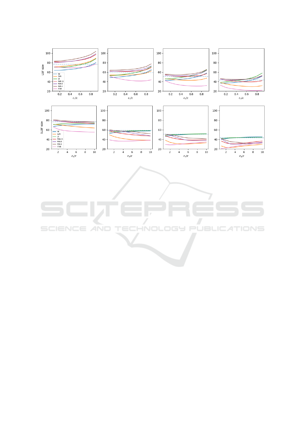
Figure 1: Size of LBF (first row) and SLBF (second row) for different classifier false positive rate. Dashed line is the size of
the corresponding Bloom Filter. From the left, figures refer to a desired false positive rate ε of 0.001, 0.005, 0.01, 0.02.
however, the SVM is very competitive, mainly when
embedded in the SLBF, being almost indistinguish-
able with FFNN in terms of space gain. Another sur-
prising result is for the LBFs with ε = 0.001, where
the NB allows the best space reduction. Such results
are even more meaningful if we consider the reject
times shown in Table 3: the filters built using SVMs
and NB are two orders of magnitude faster than those
using FFNNs. Thus, what is counterintuitive is that
non-linear or complex is not necessarily better than
linear and simple when we are declining the charac-
teristics of a classifier to be employed in a learned
Bloom Filter. It is likely such results are tied to the
size of key set, being higher the potential gain of a
learned version vs. its classic counterpart when the
number of keys increases (Dai and Shrivastava, 2020;
Ma and Liang, 2020). This is left to future investiga-
tions.
4 CONCLUSIONS AND FUTURE
DEVELOPMENTS
We have preliminarily investigated the impact of gen-
eral purpose classifiers within recently proposed ex-
tension of Bloom Filters, named learned Bloom Fil-
ters. Following (Mitzenmacher, 2018), which empha-
sized how these learned extensions are dependent on
the data distribution, we have conducted an empiri-
cal evaluation in the context of malicious URLs de-
tection, considering a wide range of general purpose
classifiers. Previous works on learned Bloom Filters
have not focused on the appropriate choice of the clas-
sifier, and simply relied on non-linear models. Our
results have confirmed the suitability of such classi-
fiers, but also have affirmed that simpler classifiers
(e.g., linear) might be the best choice in some spe-
cific contexts, especially when the reject time is also
a key factor. Future works in this directions would
extend and further validate the learned Bloom Filters
on different application domains, e.g. Genomics, Cy-
ber security, Web networking, and test the obtained
results against problems with different key set sizes
and distributions, thus allowing to unveil further in-
sights into the role played by the classifiers, possi-
bly including even those discarded in this paper for
their excessive space occupancy. Finally, the adop-
tion of succinct representations of the trained classi-
fiers, e.g. Neural Networks (Long et al., 2019; Marin
`
o
et al., 2021a; Marin
`
o et al., 2021b), might sensibly
contribute to reduce the size of a learned filter.
ACKNOWLEDGEMENTS
This work has been supported by the Italian MUR
PRIN project “Multicriteria data structures and al-
gorithms: from compressed to learned indexes, and
beyond” (Prot. 2017WR7SHH). Additional sup-
port to R.G. has been granted by Project INdAM -
GNCS Project 2020 Algorithms, Methods and Soft-
ware Tools for Knowledge Discovery in the Context
of Precision Medicine.
On the Choice of General Purpose Classifiers in Learned Bloom Filters: An Initial Analysis Within Basic Filters
681

REFERENCES
Amato, D., Giancarlo, R., and Bosco, G. L. (2021). Learned
sorted table search and static indexes in small space:
Methodological and practical insights via an experi-
mental study. CoRR, abs/2107.09480.
Bloom, B. H. (1970). Space/time trade-offs in hash cod-
ing with allowable errors. Commun. ACM, 13(7):422–
426.
Boffa, A., Ferragina, P., and Vinciguerra, G. (2021).
A “learned” approach to quicken and compress
rank/select dictionaries. In Proceedings of the SIAM
Symposium on Algorithm Engineering and Experi-
ments (ALENEX).
BOTW (2021). Best of the Web – Free Business Listing.
https://botw.org. Last checked on Oct. 18, 2021.
Broder, A. and Mitzenmacher, M. (2002). Network Appli-
cations of Bloom Filters: A Survey. In Internet Math-
ematics, volume 1, pages 636–646.
Cho, K., van Merrienboer, B., G
¨
ulc¸ehre, C¸ ., Bahdanau, D.,
Bougares, F., Schwenk, H., and Bengio, Y. (2014).
Learning phrase representations using RNN encoder-
decoder for statistical machine translation. In Proc.
of the 2014 Conf. on Empirical Methods in Natural
Language Processing, EMNLP 2014, October 25-29,
2014, Doha, Qatar, A meeting of SIGDAT, a Special
Interest Group of the ACL, pages 1724–1734. ACL.
Cortes, C. and Vapnik, V. (1995). Support-vector networks.
Machine learning, 20(3):273–297.
Cox, D. R. (1958). The regression analysis of binary se-
quences. Journal of the Royal Statistical Society: Se-
ries B (Methodological), 20(2):215–232.
Dai, Z. and Shrivastava, A. (2020). Adaptive Learned
Bloom Filter (Ada-BF): Efficient utilization of the
classifier with application to real-time information fil-
tering on the web. In Advances in Neural Information
Processing Systems, volume 33, pages 11700–11710.
Curran Associates, Inc.
Duda, R. O. and Hart, P. E. (1973). Pattern Classification
and Scene Analysis. John Willey & Sons, New Yotk.
Duda, R. O., Hart, P. E., and Stork, D. G. (2000). Pattern
Classification, 2nd Edition. Wiley.
Ferragina, P., Lillo, F., and Vinciguerra, G. (2021). On the
performance of learned data structures. Theoretical
Computer Science, 871:107–120.
Ferragina, P. and Vinciguerra, G. (2020a). Learned Data
Structures. In Recent Trends in Learning From Data,
pages 5–41. Springer International Publishing.
Ferragina, P. and Vinciguerra, G. (2020b). The PGM-index:
a fully-dynamic compressed learned index with prov-
able worst-case bounds. PVLDB, 13(8):1162–1175.
Freedman, D. (2005). Statistical Models : Theory and Prac-
tice. Cambridge University Press.
Kipf, A., Marcus, R., van Renen, A., Stoian, M., Kemper,
A., Kraska, T., and Neumann, T. (2020). Radixspline:
A single-pass learned index. In Proc. of the Third In-
ternational Workshop on Exploiting Artificial Intelli-
gence Techniques for Data Management, aiDM ’20,
pages 1–5. Association for Computing Machinery.
Kraska, T., Beutel, A., Chi, E. H., Dean, J., and Polyzotis,
N. (2018). The case for learned index structures. In
Proc. of the 2018 Int. Conf. on Management of Data,
SIGMOD ’18, pages 489–504, New York, NY, USA.
Association for Computing Machinery.
Long, X., Ben, Z., and Liu, Y. (2019). A survey of related
research on compression and acceleration of deep neu-
ral networks. Journal of Physics: Conference Series,
1213:052003.
Ma, J. and Liang, C. (2020). An empirical analysis of the
learned bloom filter and its extensions. Unpublished.
Paper and code no more available on line.
Machine Learning Lab (2021). Hidden fraudulent urls
dataset. https://machinelearning.inginf.units.it/data-
and-tools/hidden-fraudulent-urls-dataset. Last
checked on Oct. 18, 2021.
Maltry, M. and Dittrich, J. (2021). A critical analysis of
recursive model indexes. CoRR, abs/2106.16166.
Marcus, R., Kipf, A., van Renen, A., Stoian, M., Misra,
S., Kemper, A., Neumann, T., and Kraska, T.
(2020a). Benchmarking learned indexes. arXiv
preprint arXiv:2006.12804, 14:1–13.
Marcus, R., Zhang, E., and Kraska, T. (2020b). CDFShop:
Exploring and optimizing learned index structures. In
Proc. of the 2020 ACM SIGMOD Int. Conf. on Man-
agement of Data, SIGMOD ’20, pages 2789–2792.
Marin
`
o, G. C., Ghidoli, G., Frasca, M., and Malchiodi,
D. (2021a). Compression strategies and space-
conscious representations for deep neural networks.
In Proceedings of the 25th International Conference
on Pattern Recognition (ICPR), pages 9835–9842.
doi:10.1109/ICPR48806.2021.9412209.
Marin
`
o, G. C., Ghidoli, G., Frasca, M., and Malchiodi,
D. (2021b). Reproducing the sparse huffman address
map compression for deep neural networks. In Re-
producible Research in Pattern Recognition, pages
161–166, Cham. Springer International Publishing.
doi:10.1007/978-3-030-76423-4 12.
Mitzenmacher, M. (2018). A model for learned bloom fil-
ters and optimizing by sandwiching. In Advances in
Neural Information Processing Systems, volume 31.
Curran Associates, Inc.
Mitzenmacher, M. and Vassilvitskii, S. (2020). Algorithms
with predictions. CoRR, abs/2006.09123.
Python Software Foundation (2021). pickle – python object
serialization. https://docs.python.org/3/library/pickle.
html. Last checked on Oct. 18, 2021.
UNIMAS (2021). Phishing dataset. https://www.fcsit.
unimas.my/phishing-dataset. Last checked on Oct. 18,
2021.
Vaidya, K., Knorr, E., Kraska, T., and Mitzenmacher, M.
(2021). Partitioned learned bloom filters. In Interna-
tional Conference on Learning Representations.
Zell, A. (1994). Simulation neuronaler Netze. habilitation,
Uni Stuttgart.
ICPRAM 2022 - 11th International Conference on Pattern Recognition Applications and Methods
682
