Detecting Anomalies Reliably in Long-term Surveillance Systems

Jinsong Liu

, Ivan Nikolov

, Mark P. Philipsen

and Thomas B. Moeslund

Visual Analysis and Perception Laboratory, CREATE, Aalborg University, 9000 Aalborg, Denmark

Keywords:

Surveillance, Anomaly Detection, Autoencoder, Long-term, Weighted Reconstruction Error, Background

Estimation.

Abstract:

In surveillance systems, detecting anomalous events like emergencies or potentially dangerous incidents by

manual labor is an expensive task. To improve this, anomaly detection automatically by computer vision

relying on the reconstruction error of an autoencoder (AE) is extensively studied. However, these detection

methods are often studied in benchmark datasets with relatively short time duration — a few minutes or

hours. This is different from long-term applications where time-induced environmental changes impose an

additional inﬂuence on the reconstruction error. To reduce this effect, we propose a weighted reconstruction

error for anomaly detection in long-term conditions, which separates the foreground from the background and

gives them different weights in calculating the error, so that extra attention is paid on human-related regions.

Compared with the conventional reconstruction error where each pixel contributes the same, the proposed

method increases the anomaly detection rate by more than twice with three kinds of AEs (a variational AE,

a memory-guided AE, and a classical AE) running on long-term (three months) thermal datasets, proving the

effectiveness of the method.

1 INTRODUCTION

For a safer daily life, round-the-clock surveillance

systems have been installed in some private and pub-

lic places. Generally they are manually operated,

which is expensive. Therefore, an automatic tool to

help ﬁnd emergencies or potentially dangerous inci-

dents that require extra attention is in dire needed.

From the perspective of computer vision, such a

tool can be realized using either supervised or un-

supervised learning. Supervised learning needs a

large amount of annotated data illustrating what the

emergencies or potentially dangerous incidents look

like. This is too expensive as collecting enough data

of rarely-occurring incidents is time consuming and

even unfeasible. On the contrary, unsupervised learn-

ing greatly lowers the cost, making it more preferred

in this task.

This unsupervised solution is often realized

by anomaly detection via an autoencoder (AE),

which treats these rarely-happening emergencies and

potentially dangerous incidents as anomalies but

https://orcid.org/0000-0002-5231-6950

https://orcid.org/0000-0002-4952-8848

https://orcid.org/0000-0002-9212-2544

https://orcid.org/0000-0001-7584-5209

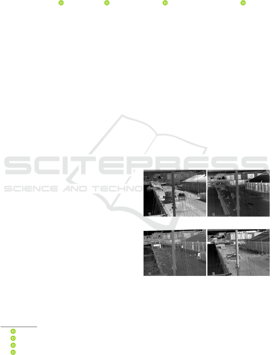
(a) August (b) January

Figure 1: Example images from different months. All show

normal activity but with signiﬁcant differences due to the

seasons.

frequently-occurring incidents as normal. In general,

an anomaly is deviating from a normal in many as-

pects. An AE trained with only normal data can re-

construct similar normal patterns with minimal errors,

but struggles with abnormal patterns. Hence the dif-

ference between the input and the reconstructed out-

Liu, J., Nikolov, I., Philipsen, M. and Moeslund, T.

Detecting Anomalies Reliably in Long-term Surveillance Systems.

DOI: 10.5220/0010907000003124

In Proceedings of the 17th International Joint Conference on Computer Vision, Imaging and Computer Graphics Theory and Applications (VISIGRAPP 2022) - Volume 4: VISAPP, pages

999-1009

ISBN: 978-989-758-555-5; ISSN: 2184-4321

999

put, usually in the form of mean square error (MSE),

has the ability to measure the input’s deviation from

the normal data. Input with the MSE larger than a

predeﬁned threshold is detected as an anomaly.

This detection strategy works with an assumption

that the concept of what is normal is constant. Bench-

mark datasets on which existing anomaly detection

solutions are evaluated satisfy this assumption, be-

cause they are relatively short in time duration. How-

ever, in real life a surveillance system will be run-

ning for months and hence the normal pattern will

inevitably drift. This can be illustrated in Figure 1

where all these four harbor front scenes are normal

in terms of human activities, but the obvious changes

across time in contrast, illumination, water ripples,

and other environmental aspects make them different

from what has been deﬁned as normal in the training

phase. This time-induced drift has a large inﬂuence

on the reconstruction error and thus the anomaly de-

tection is not reliable any more. This phenomenon

raises an open research question — how to detect

anomalies reliably in long-term surveillance systems.

To this end, we propose a weighted reconstruc-

tion error method that uses different weights for

foreground pixels and background pixels in calculat-

ing the error, for which ﬁve background estimation

(foreground extraction) methods are implemented and

evaluated. In this way, the inﬂuence of the time-

induced drift on the reconstruction error is reduced

and hence anomaly detection is more reliable.

By applying the proposed method to long-term

datasets spanning three months (August 2020, Jan-

uary 2021, April 2021) collected from a real-world

harbor front surveillance system, the experimental re-

sults show that the weighted reconstruction error in-

creases the anomaly detection rate by at least twice

than that with the conventional reconstruction error,

for all the three kinds of AEs (a variational AE, a

memory-guided AE, and a classical AE), proving the

effectiveness of the method.

The datasets and code are published on GitHub —

https://github.com/JinsongCV/Weighted-MSE, mak-

ing the integration of the weighted reconstruction er-

ror and the comparison between before and after re-

sults much easier.

2 RELATED WORK

Existing work on anomaly detection (Hasan et al.,

2016; Chong and Tay, 2017; Fu et al., 2018; Yue et al.,

2019; Nguyen and Meunier, 2019; Song et al., 2019;

Gong et al., 2019; Deepak et al., 2020; Tsai and Jen,

2021; Liu et al., 2021b) is usually AE-based.

Table 1: Time duration (hours) of benchmark datasets for

anomaly detection.

Avenue ShanghaiTec UCSD UMN Subway

0.5 3.6 3.1 0.07 2.3

Though some attempts are made to improve the

anomaly detection performance, for example incor-

porating temporal information (Fu et al., 2018; Yue

et al., 2019; Nguyen and Meunier, 2019), introducing

a generative adversarial network (GAN) to differen-

tiate reconstructions from inputs (Song et al., 2019),

using both the memorized features of the training set

and the input’s features to do reconstruction (Gong

et al., 2019; Park et al., 2020), and so on, these meth-

ods are only studies on benchmark datasets — Avenue

(Lu et al., 2013), ShanghaiTech (Luo et al., 2017),

UCSD (Mahadevan et al., 2010), UMN (Mehran

et al., 2009), and Subway (Adam et al., 2008)), which

have an imperfection in common — a short duration

of a few minutes or hours (shown in Table 1) (Pranav

et al., 2020; Nikolov et al., 2021). Therefore, gener-

alizing the existing work evaluated on such datasets

to a long-term application in real life can be problem-

atic, considering the extra time-induced changes. For

example, the illumination and contrast vary from the

shifts in day and night, weather, seasons, etc. This en-

vironmental drift imposes an additional variation on

the reconstruction error and thus makes it not solely

correlated to human activities that are responsible for

most anomalies.

This challenge inspires us to focus more on fore-

ground regions where anomalies are assumed in when

calculating the reconstruction error, to eliminate the

inﬂuence of the time-induced environmental drift,

which is exactly the proposed weighted reconstruc-

tion error does.

A similar solution to ours is the object-centric

AE (Ionescu et al., 2019; Georgescu et al., 2020)

that takes the pre-detected object region instead of

the full image as the input. Despite the similarity,

there are four distinctions. (i) The goals are differ-

ent. Their work expects to generalize an AE trained

on one scene to another scene without further ﬁnetun-

ing, while our method targets to reduce the effect of

the environmental drift in long-term surveillance sys-

tems. (ii) Our method still reconstructs the full image

instead of only object regions, because the location of

an object relative to the background is important, for

example, a drowning accident only happens in the wa-

ter area. (iii) Our method is much more ﬂexible like a

post-processing module and thus easily incorporated

to any framework. (iv) Our method treating fore-

ground and background regions separately also pro-

vides an ability to investigate environmental anoma-

VISAPP 2022 - 17th International Conference on Computer Vision Theory and Applications

1000

lies like a sudden contrast change due to an extreme

weather event.

3 METHODS

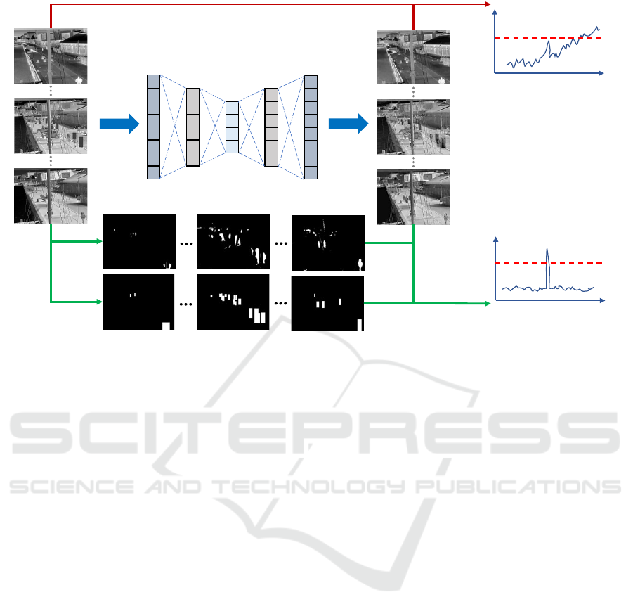
This paper proposes a weighted reconstruction error

for anomaly detection illustrated by the diagram in

Figure 2.

In it, the red ﬂow indicates the conventional

anomaly detection scheme where the reconstruction

error (in the form of MSE) is directly calculated from

the input and the reconstructed output with each pixel

contributes the same. This calculation also considers

the time-induced environmental drift as part of the re-

construction error, and thus for input spanning a long

time period the MSE curve will ﬂuctuate greatly. This

is very dangerous as a real anomaly will be ignored, if

its MSE value is lower than other ﬂuctuated MSE val-

ues of normal inputs. Such a phenomenon is shown in

the upper MSE curve where normal inputs with drift

have larger MSE values than the threshold (the red

dashed line), not only introducing false positives but

also missing the real anomaly.

In contrast, the green ﬂow in the diagram in-

dicates the proposed weighted reconstruction error-

based anomaly detection scheme. Additional back-

ground estimators or object-centric foreground ex-

tractors can segment an input into foreground region

and background region. This information together

with the input and the reconstruction are used to cal-

culate the reconstruction error where the foreground

pixels and background pixels are assigned different

weights, so that the error focuses more on the region

where anomalies usually happen and thus the effect

of the environmental drift is reduced. In this way,

the weighted MSE curve will be much more smoother

for normal inputs but generates a peak if an anomaly

comes in, like the lower W-MSE curve shows. An-

other thing to be mentioned is that both the red ﬂow

scheme and the proposed green ﬂow scheme are indi-

cating the inference phase — anomaly detection.

3.1 Autoencoder

Following what is customary, we use an AE to de-

tect anomalies by ﬁnding frames with the largest re-

construction errors. Three AEs are applied. The

ﬁrst is a variational AE — VQVAE2 (Razavi et al.,

2019) whose encoder compresses the input into multi-

scale quantized latent maps for the decoder to process.

The second is a memory-guided AE — MNAD (Park

et al., 2020) that uses a concatenated latent space (of

the naive latent space from the encoder output and

the typical features stored in a memory module con-

structed from training) to reconstruct the input. An

anomaly is measured by not only the reconstruction

error but also the distance between the encoder out-

put and the nearest memorized features. The third is

a classical AE (CAE) designed by us, which is with-

out any advanced processing of the latent space. This

CAE uses eleven convolution layers and ﬁve pooling

layers to downsize the input (384 × 288 × 1) into a

compressed feature tensor (10 × 7 × 64), and another

six transposed convolution layers and ﬁve convolu-

tion layers to transform the latent feature space into

the reconstructed output. Detailed implementations

are shared on GitHub.

3.2 Background Estimation

As mentioned before, the method is characteristic of

foreground regions and background regions contribut-

ing differently to the weighted reconstruction error.

Therefore, separating the background from the fore-

ground is the key. To achieve this we test out two

pipelines, one using classical statistical methods to es-

timate the background, the other one using the result

of a human detector as the foreground and everything

else as the background.

In section 4, we will test all the methods of the

two pipelines and determine which is the best method

or the best combination of a few methods to separate

the foreground from the background, so that the drift

can be removed effectively for improving the anomaly

detection rate.

3.2.1 Statistical Background Estimation

This pipeline is composed of classical statistical ap-

proaches instead of deep learning segmentation meth-

ods (Babaee et al., 2018; Akilan et al., 2019) to min-

imize the complexity. Also this avoids the high price

of supervised segmentation concerning pixel-level an-

notations. In our harbor front scenario, the objects

in the foreground vary signiﬁcantly — humans from

a single one to groups, vehicles, bicycles, and oth-

ers. These variations cause extra difﬁculties and man-

power in pixel-level annotations if a deep model is

chosen. The four classical background estimators are

as follows:

• Mixture of Gaussians (MOG2) (Zivkovic, 2004)

— using Gaussian mixture probability density to

continuously model the background.

• Mixture of Gaussians using K-nearest neighbours

(KNN) (Zivkovic and Van Der Heijden, 2006) —

an extension of the MOG2 method by implement-

Detecting Anomalies Reliably in Long-term Surveillance Systems

1001

Input

time

MSE

time

W-MSE

Autoencoder

Background Estimators

Object-centric Foreground

Extractors

econstruction

Anomaly

Figure 2: Diagram of the proposed method.

ing a K-nearest neighbours algorithm on top for a

more robust kernel density estimation.

• Image difference with arithmetic mean (ID

) —

the difference between the current image and the

previous one is processed by adaptive threshold-

ing to get the background mask. ID

uses an arith-

metic mean weight — each pixel in the neigh-

borhood contributes equally to compute the local

threshold.

• Image difference with Gaussian mean (ID

) — the

same principle with ID

, but with a different adap-

tive thresholding strategy. ID

uses a Gaussian

mean weight — pixels in the neighborhood far-

ther away from the center contribute less to the

local threshold computing.

To do background estimation, all the four methods

need the neighbouring images of the current frame.

For the MOG2 and KNN methods, the number of

neighbouring images is heuristically set to 20, as it

has been shown that more frames are better at mod-

eling the background. For the ID

and ID

methods,

only one previous image is used.

Once a mask is acquired from any of the four

methods, it goes through a post-processing procedure

— a morphological closing with a structuring element

of size 7 × 7 followed by an opening with an ele-

ment of size 3 × 3. This step serves to remove small

noise particles. Finally, the moving elements in the

background like the water, ropes, and masts are re-

moved from the mask by prior knowledge of their lo-

cations. The resulting mask will have foreground pix-

els with large grayscale values approaching 255 and

background pixels with small values near 0. All of

these procedures are implemented from the OpenCV

library (Bradski, 2000).

3.2.2 Object-centric Foreground Extraction

Besides the above four classical approaches, we test

another method — object-centric foreground extrac-

tion, provided that there is a well-trained human de-

tector at hand and human activities are the targets.

The detector we use is YOLOv5 (Ultralytics, 2020;

Liu et al., 2021a), with which each person is repre-

sented by a rectangle in the mask. The pixels in the

rectangle has a same grayscale value — the person’s

detection conﬁdence multiplied by 255, while pixels

in other regions are with the value 0.

As a whole, these ﬁve versions of masks explicitly

locate foreground areas with very large grayscale val-

ues, so for a clear reference the subsequent contents

will call such a mask foreground map. Figure 3 shows

one input image and the results from the ﬁve methods.

3.3 Weighted Reconstruction Error

First to be noted is that this paper goes with the con-

vention and thus opts for the MSE to measure the dif-

ference between the input and the reconstructed out-

put, so the following contents will directly use MSE to

represent the difference without further explanation.

VISAPP 2022 - 17th International Conference on Computer Vision Theory and Applications

1002

(a) Input (b) MOG2 (c) KNN (d) ID

(e) ID

(f) YOLOv5

Figure 3: An input thermal image and the outputs from the ﬁve implemented background estimation (foreground extraction)

methods.

As long as there is a foreground map M locating

foreground pixels P

f g

, any weighted MSE is possible

by giving P

f g

and background pixels P

arbitrarily-

deﬁned weights for a speciﬁc task.

For an input I with size H ×W and its correspond-

ing reconstruction R, a general weighted MSE

is:

MSE

∑

i=1

∑

j=1

i j

− R

i j

)

H ×W

(1)

where

i j

is the value of the weight map

M at pixel

(i, j).

M is calculated using Equation 2.

M =

f g

× M + w

× (255 − M)

255

(2)

where w

f g

and w

are normalized weights for P

f g

and P

, respectively; as an 8-bit image, 255 − M is

the “inverse” operation of M, explicitly locating P

;

therefore

M is the ﬁnal weight map normalized to 0-1

for calculating weighted MSE in Equation 1.

Setting w

f g

as 1 and w

as 0 is the special case of

the MSE only considering P

f g

. Likewise, setting w

f g

as 0 and w

as 1 is the MSE only looking at P

A more general case is a weighted MSE

com-

bining foreground maps (e.g., M

, M

) from several

background estimators (foreground extractors).

MSE

∑

i=1

∑

j=1

i j

− R

i j

)

H ×W

(3)

M = w

+ w

(4)

f g

× M

+ w

× (255 − M

)

255

(5)

f g

× M

+ w

× (255 − M

)

255

(6)

where,

is the weight map from M

with w

f g

and

as normalized weights for P

f g

and P

in M

;

is the weight map from M

with w

f g

and w

as nor-

malized weights for P

f g

and P

in M

;

M is the ﬁnal

weight map combining

with weight w

and

with weight w

; the resulting MSE

is the weighted

MSE considering foreground maps from two meth-

ods.

4 EXPERIMENTS

4.1 Dataset Information

Two datasets collected from a long-term harbor front

surveillance system are used to investigate the pro-

posed weighted MSE on anomaly detection.

One dataset called 300Ver has 300 images with

every 100 sampled from August 2020, January 2021,

and April 2021, making itself a dataset spanning 76

days. This dataset is a subset of a larger one covering

8-month and publicly available as part of the publica-

tion (Nikolov et al., 2021). The sampling protocol for

300Ver is also given in (Nikolov et al., 2021) which

uses the temperature as a basis to construct datasets

covering cold, warm, and in-between months.

The other dataset called 3515Ver is also a subset

of the dataset from (Nikolov et al., 2021), and has

3515 images intensively sampled with a frame rate of

0.5fps from 15 pm to 18 pm from 14-16 August 2020,

14-16 January 2021, and 14-16 April 2021. This sam-

pling protocol comes from three strategies. (i) Em-

pirically 15 pm to 18 pm is the time period when

there are most people present in view. (ii) Three days

from each month not only guarantee the data diversity

across time but also limit the amount of the dataset for

better visualization in section 4.3.3. (iii) 0.5fps limits

the amount of 3515Ver, at the same time keeping the

information continuity between neighboring frames.

In 300Ver persons are annotated with bounding

boxes. Therefore, six foreground maps from MOG2,

KNN, ID

, ID

, YOLOv5, and ground truth (GT), are

prepared for each image. The 3515Ver dataset has

no such annotations, so only ﬁve kinds of foreground

maps are calculated.

First the 300Ver dataset is used and the related

experiments are in sections 4.3.1 and 4.3.2. The

3515Ver dataset is then used to verify what has been

found on 300Ver and the related contents are in sec-

tion 4.3.3. There are three reasons why we do ex-

periments on both datasets. (i) 300Ver covers 76 days

with less images while 3515Ver have more images but

only covering 9 days; these two datasets compensate

for each other, making the experiments consider both

Detecting Anomalies Reliably in Long-term Surveillance Systems

1003

a long-term duration and a large amount of images.

(ii) This separation of two datasets avoids the prob-

lem that if all the images are sampled intensively from

the 76 days, the resultant 30000 images will make the

visualization of drawing the MSE values of them into

one curve (like the curve in the following contents)

extremely difﬁcult. (iii) Annotating a small dataset

(300Ver) is much easier to provide a very accurate

foreground extraction, based on which the ﬁndings of

section 4.3.1 will be more convincing.

4.2 Implementation Details

Both VQVAE2 and MNAD are trained with 4000 im-

ages and validated with 1000 images. CAE is trained

with 15000 images and validated with 5000 images

due to its naive function compared with the other two.

VQVAE2 is trained with a batch size of 32 and a

learning rate of 0.0001. MNAD is trained with a batch

size of 32, a learning rate of 0.0002, and a value of 0.1

for the weight of the feature separateness and com-

pactness loss. CAE is trained with a batch size of 16

and a learning rate of 0.0003. The training phases stop

at the 100th epoch, the 100th epoch, and the 200th

epoch for VQVAE2, MNAD, and CAE, respectively,

at which the networks are converged with the train-

ing losses not decreasing any more. All these training

and validation sets are sampled from February 2021 to

not only avoid the overlapping with the three-month

datasets this paper uses but also enhance the effect of

the time-induced drift that we want to address. A kind

reminder is that the following experiments are done

with all these three AEs but we usually only show re-

lated visualizations of VQVAE2 to avoid the repeat of

similar results.

The YOLOv5 detector uses a pretrained model

from (Liu et al., 2021a) and the training set has no

overlapping with the images we use in this paper.

4.3 Weighted MSE

4.3.1 Weighted MSE Curves

To simplify the work and directly answer the ques-

tion how the conventional MSE and weighted MSE

behave for long-term datasets, according to Equation

1 and Equation 2, the MSE investigated will consider

three situations: the foreground only, the background

only, and the full image where each pixel contributes

the same as the convention, which are represented as

MSE

f g

, MSE

cvt

, respectively. These repre-

sentations will be used in all the following contents.

Therefore, for each AE with 300Ver as input, six

kinds of foreground maps produce six MSE

f g

curves

and six MSE

curves describing the weighted MSE

changes across time; likewise, one MSE

cvt

curve can

be drawn to describe the conventional MSE changes

across time.

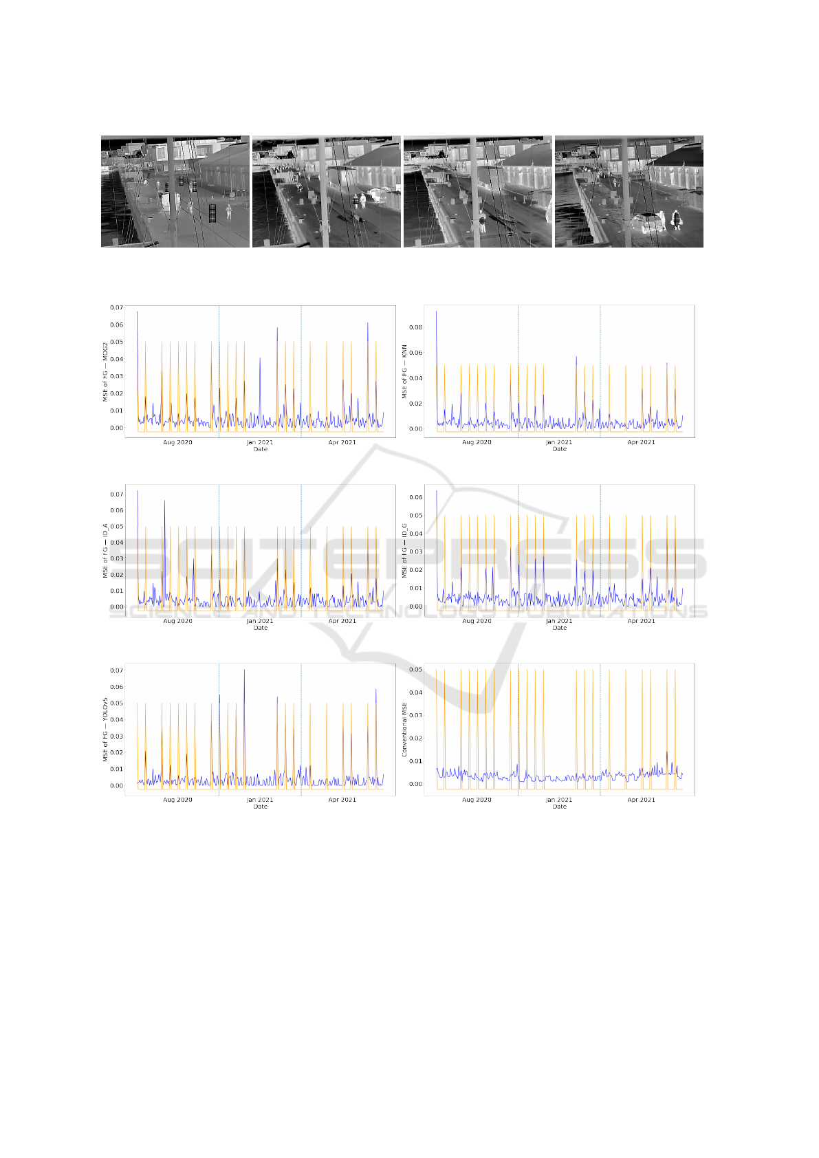
For a better comparison, Figure 4 shows the above

mentioned 13 MSE curves, produced by the VQVAE2

model. This visualization (of showing multiple curves

in one chart) is achieved with a critical pre-processing

module before plotting: ﬁrst the original MSE val-

ues are smoothed by a mean ﬁlter with its kernel size

as 10; then the smoothed values are normalized be-

tween 0 and 1; after normalization the curves are

overlapped with each other, so a further translation is

done for each curve by adding an extra value. In this

way, the ranges of curves of MOG2, KNN, ID

, ID

YOLOv5, and GT are [2.5, 3.5], [2.0, 3.0], [1.5, 2.5],

[1.0, 2.0], [0.5, 1.5], [0, 1], respectively; the range of

the conventional MSE curve is [3.0, 4.0].

From Figure 4 several observations are found. (i)

The six MSE

f g

curves in (a) have totally different

trends with the trends of MSE

curves in (b), which

is reasonable as the image regions they look at are

not the same. (ii) The MSE

cvt

curve in (b) has al-

most exactly same trend with that of the six MSE

curves in (b), but largely deviates from the trends of

MSE

f g

curves in (a), proving that on 300Ver the con-

ventional MSE (where each pixel in the full image

contributes the same) cannot represent what happens

in the foreground region and thus have no ability to

do anomaly detection reliably. (iii) Though the six

MSE

f g

curves in (a) are diverse, they share a similar

trend to some extent especially between the MSE

f g

curve of YOLOv5 and the MSE

f g

curve of GT. This

reﬂects that they have the ability to represent the fore-

ground changes along with time but also have their

own focuses shown by distinct peaks due to the meth-

ods’ differences. The MSE

f g

curve of YOLOv5 and

the MSE

f g

curve of GT are bounding box-based fo-

cusing only on persons, therefore a larger similarity

is found between them. (iv) The trends of all the

MSE

curves and the MSE

cvt

curve in (b) are U-

shape, revealing the inﬂuence of the drift across time

on the MSE as mentioned before. However, the U-

shape trend is not shown in foreground MSE curves in

(a), indicating that the time-induced effect inﬂuences

background regions higher than foreground regions.

Hence researches on long-term datasets (applications)

need separate analysis on them.

In addition to this, experiments done with MNAD

and CAE also get similar results that all support the

above ﬁndings. As a whole, this part conﬁrms that in

long-term datasets (applications) with time-induced

drift, the conventional MSE (where each pixel con-

tributes the same) is not suitable to describe the fore-

VISAPP 2022 - 17th International Conference on Computer Vision Theory and Applications

1004

(a) MSE

f g

(b) MSE

and MSE

cvt

Figure 4: MSE (after smoothing, normalization, and translation) curves across time from VQVAE2 on 300Ver. The vertical

azure dashed lines are used to separate different months.

ground information, not to mention a further step —

detecting anomalies.

4.3.2 Weighted MSE for Anomaly Detection

This section will test whether the proposed weighted

MSE performs better in anomaly detection. Since

there are no speciﬁed anomalies in the dataset, and

detecting speciﬁc anomalies is not the focus of this

work, we decide to use a strategy that maximizes

the difference between an anomaly and a normal im-

age, to better focus on the main research problem —

how to do anomaly detection reliably in long-term

datasets.

To realize this, we synthesize anomalies by over-

lapping “black-white-pixel” patterns (that the three

AEs have never seen) on the person regions of some

images. But it seems that such patterns overlapped

on only person regions will give the YOLOv5-based

foreground map a biased advantage. Hence, to eval-

uate the ﬁve kinds of foreground maps more fairly,

four shapes (rectangle, square, circle, and ellipse)

of the “black-white-pixel” pattern are considered for

the reason that the detector-based map has no round-

cornered foregrounds but the other four kinds of

maps have. We admit this four-shape strategy can-

not totally remove the bias on the YOLOv5-generated

map, but if we put the “black-white-pixel” pattern

on other foreground regions where there are no peo-

ple, a greater bias will be given to other statistical

background estimators because YOLOv5 only pre-

dicts human regions. Therefore, this four-shape strat-

egy should be the best solution to treat these ﬁve kinds

of foreground maps equally.

Accordingly, on the premise of having at least

one person in each synthesized anomalous image, 21

rectangle-shaped anomalies (the 1st, 11st, 21st, ...,

281st images of 300ver), 21 square-shaped anoma-

lies (the 3rd, 13rd, ..., 293rd images of 300ver), 20

circle-shaped anomalies (the 2nd, 12nd, ..., 282nd im-

ages of 300ver), and 16 ellipse-shaped anomalies (the

4th, 14th, ..., 284th images of 300ver) are synthesized.

In each of them the annotated GT person regions are

randomly chosen to be overlapped with “black-white-

pixel” patterns. Examples of the synthesized anoma-

lies are shown in Figure 5.

First, the rectangle-shaped anomalies are used to

test the anomaly detection rate. Accordingly, in Fig-

ure 6, six MSE curves (ﬁve MSE

f g

curves and one

MSE

cvt

curve) of VQVAE2 are drawn in color blue,

and the anomalies are located with orange peaks.

Each sub-ﬁgure caption has the same meaning with

what has been used in section 4.3.1.

From Figure 6, the large percentage of overlap-

ping between orange peaks and blue peaks in (a)-(e)

proves the usefulness of the proposed weighted MSE

in anomaly detection. This also happens in the exper-

iments of VQVAE2 on 300Ver but with anomalies in

the other three shapes. Speciﬁcally, among the images

of the largest 30 (10% of the dataset) MSE values of

each curve, the number of anomalies is listed in Table

2. From the table, the weighted MSE using any fore-

ground map has a way high detection rate than the

conventional MSE.

When taking multiple foreground maps from dif-

ferent methods into consideration, the top two results

in Table 2 — YOLOv5 and KNN, inspire us to com-

bine their foreground maps by applying Equation 3-6

in which w

(namely w

Y OLOv5

) and w

(namely w

KNN

)

are 0.52 and 0.48, respectively as the normalized val-

ues of 78.21% and 71.79%. To be noted is that any

combination is possible no matter whether a super-

vised human detector is available.

To avoid being one-sided, we do further experi-

ments with MNAD and CAE on 300Ver in a way of

using rectangle-shaped anomalies and the foreground

map combining YOLOv5 and KNN. By using the

weighted MSE instead of the conventional MSE, the

detection rate increases from 9.52% to 66.67% for

MNAD and from 4.76% to 66.67% for CAE.

Detecting Anomalies Reliably in Long-term Surveillance Systems

1005

(a) Rectangle (b) Square (c) Circle (d) Ellipse

Figure 5: Examples of anomalies with “black-white-pixel” patterns in four different shapes.

(a) MSE

f g

of MOG2 (b) MSE

f g

of KNN

f g

of ID

(d) MSE

f g

of ID

(e) MSE

f g

of YOLOv5 (f) MSE

cvt

Figure 6: After introducing rectangle-shaped anomalies, MSE curves across time from VQVAE2 on the 300Ver dataset. The

blue curves describe the MSE changes, and the orange peaks indicate the locations of anomalies. The vertical azure dashed

lines are used to separate different months.

As a whole, the proposed weighted MSE im-

proves anomaly detection rate markedly on 300Ver —

VQVAE2 (2.68 times-3.21 times), MNAD (7 times),

CAE (14 times), verifying that this strategy is worth

being incorporated in datasets or applications span-

ning a long time period.

4.3.3 Extended Experiments

The extended experiments on 3515Ver use rectangle-

shaped “black-white-pixel” patterns overlapping on

the persons who are near the horizontal edge of the

water to simulate the anomalies. The resultant 60

VISAPP 2022 - 17th International Conference on Computer Vision Theory and Applications

1006

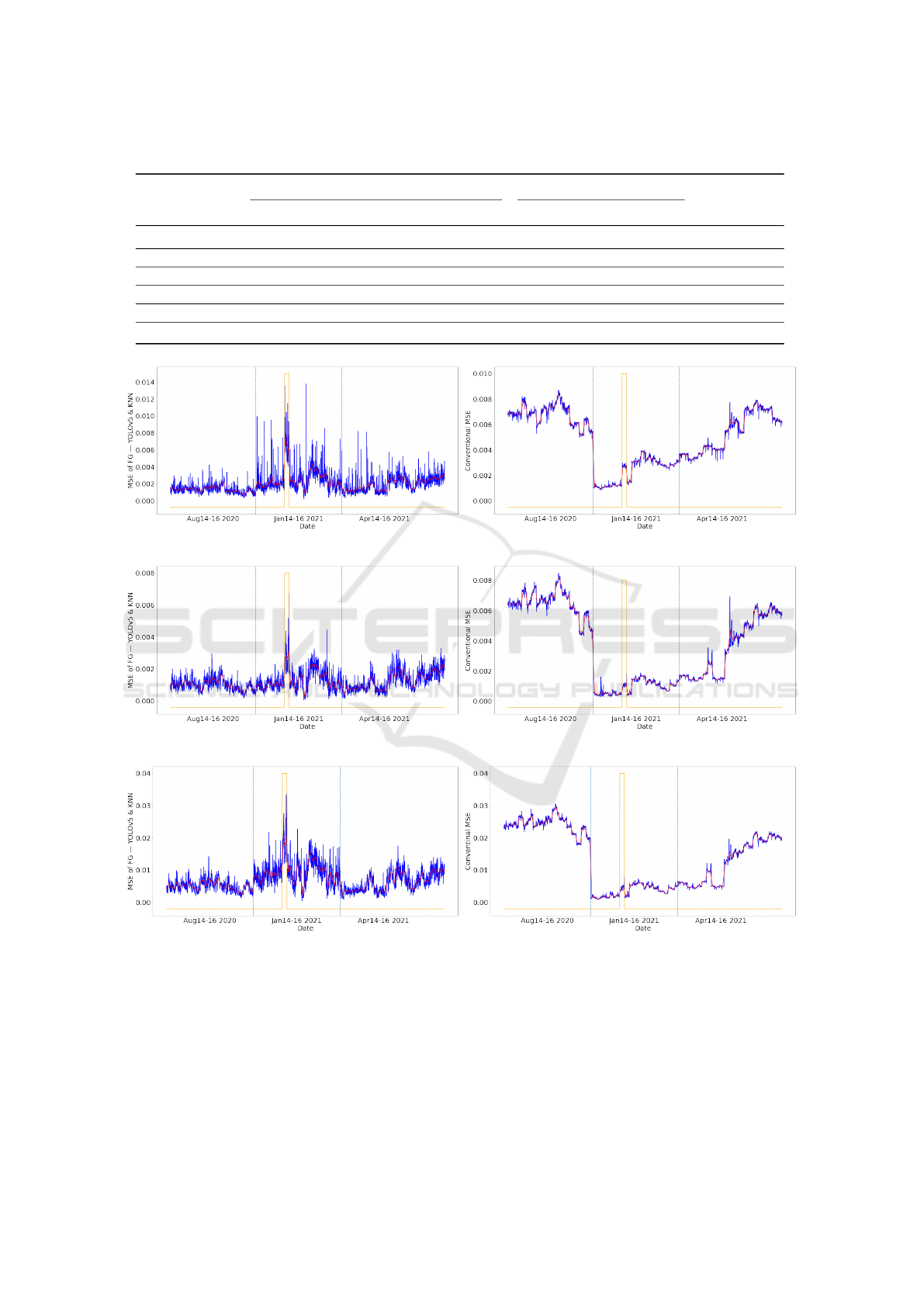
Table 2: Anomaly detection results of weighted MSE and conventional MSE.

Statistical Background Object-centric Foreground

Conventional

MOG2 KNN ID

YOLOv5

Rectangle (21) 16 17 15 15 16 4

Square (21) 13 14 12 13 15 7

Circle (20) 11 13 10 10 16 4

Ellipse (16) 14 12 14 13 14 4

Sum (78) 54 56 51 51 61 19

Detection Rate 69.23% 71.79% 65.38% 65.38% 78.21% 24.36%

(a) VQVAE2: MSE

f g

of M

Y OLOv5&KNN

(b) VQVAE2: MSE

cvt

f g

of M

Y OLOv5&KNN

(d) MNAD: MSE

cvt

(e) CAE: MSE

f g

of M

Y OLOv5&KNN

(f) CAE: MSE

cvt

Figure 7: MSE curves of VQVAE2, MNAD, and CAE on 3515Ver with synthesized rectangle-shaped anomalies. The curve

of absolute MSE values is in blue. The curve of the smoothed values are in red. The anomalies are located with orange peaks.

The vertical azure dashed lines are used to separate different months.

synthesized anomalies are consecutive frames and

the persons overlapped with the abnormal pattern are

ﬁxed individuals. This increases the authenticity of

the simulated anomalies — in real life an anomaly

usually persists through multiple frames and involves

ﬁxed persons.

Figure 7 gives the MSE curves of the three AEs

on 3515Ver with synthesized anomalies, in which

the curves of absolute MSE values are in blue and

the smoothed ones are in red, and the anomalies

Detecting Anomalies Reliably in Long-term Surveillance Systems

1007

are located with orange peaks. In Figure 7, by

using the weighted MSE with the foreground map

Y OLOv5&KNN

combining YOLOv5 and KNN, the as-

cending peaks in (a), (c), and (e) accurately detect the

anomalies, yet the conventional MSE curves in (b),

(d), and (f) are entirely dominated by time-induced

inﬂuences for example the fall of a cliff due to the

seasonal transition between August 2020 and January

2021. We therefore believe that the extended experi-

ments on a much larger dataset also prove the effec-

tiveness of the proposed weighted MSE in anomaly

detection.

5 CONCLUSIONS

This paper proposes a weighted reconstruction er-

ror in autoencoder-based anomaly detection for long-

term surveillance systems. The method aims to make

the calculated error more focused on the region where

anomalies are assumed in and thus reduces the inﬂu-

ence of time-induced environmental drift.

We apply three selected autoencoders to three-

month datasets to test the anomaly detection per-

formance. With synthesized anomalies, the autoen-

coder with proposed weighted reconstruction error al-

ways gets a much higher detection rate (more than

twice) than the conventional reconstruction error ver-

sion where each pixel contributes the same, which

proves the usefulness of the proposed strategy.

This method is implemented as a ﬂexible module,

therefore we expect it can be integrated into and veri-

ﬁed by more frameworks. Besides, as a study at har-

bor fronts, in the future we will use this method to de-

tect emergencies and potentially dangerous incidents

like trafﬁc accidents, drowning accidents, crowds in

coronavirus days, etc., so that timely controls or res-

cues by polices, safeguards, and other professionals

can be provided for a safer life.

ACKNOWLEDGEMENTS

This work is funded by TrygFonden as part of the

project Safe Harbor.

REFERENCES

Adam, A., Rivlin, E., Shimshoni, I., and Reinitz, D. (2008).

Robust real-time unusual event detection using mul-

tiple ﬁxed-location monitors. IEEE transactions on

pattern analysis and machine intelligence, 30(3):555–

560.

Akilan, T., Wu, Q. J., Safaei, A., Huo, J., and Yang, Y.

(2019). A 3d cnn-lstm-based image-to-image fore-

ground segmentation. IEEE Transactions on Intelli-

gent Transportation Systems, 21(3):959–971.

Babaee, M., Dinh, D. T., and Rigoll, G. (2018). A deep con-

volutional neural network for video sequence back-

ground subtraction. Pattern Recognition, 76:635–649.

Bradski, G. (2000). The OpenCV Library. Dr. Dobb’s Jour-

nal of Software Tools.

Chong, Y. S. and Tay, Y. H. (2017). Abnormal event detec-

tion in videos using spatiotemporal autoencoder. In

International Symposium on Neural Networks, pages

189–196. Springer.

Deepak, K., Chandrakala, S., and Mohan, C. K. (2020).

Residual spatiotemporal autoencoder for unsuper-

vised video anomaly detection. Signal, Image and

Video Processing, pages 1–8.

Fu, J., Fan, W., and Bouguila, N. (2018). A novel approach

for anomaly event detection in videos based on au-

toencoders and se networks. In 2018 9th International

Symposium on Signal, Image, Video and Communica-

tions (ISIVC), pages 179–184. IEEE.

Georgescu, M.-I., Tudor Ionescu, R., Shahbaz Khan, F.,

Popescu, M., and Shah, M. (2020). A scene-agnostic

framework with adversarial training for abnormal

event detection in video. arXiv e-prints, pages arXiv–

2008.

Gong, D., Liu, L., Le, V., Saha, B., Mansour, M. R.,

Venkatesh, S., and Hengel, A. v. d. (2019). Memoriz-

ing normality to detect anomaly: Memory-augmented

deep autoencoder for unsupervised anomaly detec-

tion. In Proceedings of the IEEE/CVF International

Conference on Computer Vision, pages 1705–1714.

Hasan, M., Choi, J., Neumann, J., Roy-Chowdhury, A. K.,

and Davis, L. S. (2016). Learning temporal regularity

in video sequences. In Proceedings of the IEEE con-

ference on computer vision and pattern recognition,

pages 733–742.

Ionescu, R. T., Khan, F. S., Georgescu, M.-I., and Shao,

L. (2019). Object-centric auto-encoders and dummy

anomalies for abnormal event detection in video. In

Proceedings of the IEEE/CVF Conference on Com-

puter Vision and Pattern Recognition, pages 7842–

7851.

Liu, J., Philipsen, M. P., and Moeslund, T. B. (2021a). Su-

pervised versus self-supervised assistant for surveil-

lance of harbor fronts. In VISIGRAPP (5: VISAPP),

pages 610–617.

Liu, J., Song, K., Feng, M., Yan, Y., Tu, Z., and Zhu,

L. (2021b). Semi-supervised anomaly detection

with dual prototypes autoencoder for industrial sur-

face inspection. Optics and Lasers in Engineering,

136:106324.

Lu, C., Shi, J., and Jia, J. (2013). Abnormal event detection

at 150 fps in matlab. In Proceedings of the IEEE inter-

national conference on computer vision, pages 2720–

2727.

Luo, W., Liu, W., and Gao, S. (2017). In Proceedings of the

IEEE International Conference on Computer Vision,

pages 341–349.

VISAPP 2022 - 17th International Conference on Computer Vision Theory and Applications

1008

Mahadevan, V., Li, W., Bhalodia, V., and Vasconcelos, N.

(2010). Anomaly detection in crowded scenes. In

2010 IEEE Computer Society Conference on Com-

puter Vision and Pattern Recognition, pages 1975–

1981. IEEE.

Mehran, R., Oyama, A., and Shah, M. (2009). Abnormal

crowd behavior detection using social force model. In

2009 IEEE Conference on Computer Vision and Pat-

tern Recognition, pages 935–942. IEEE.

Nguyen, T.-N. and Meunier, J. (2019). Anomaly detection

in video sequence with appearance-motion correspon-

dence. In Proceedings of the IEEE International Con-

ference on Computer Vision, pages 1273–1283.

Nikolov, I. A., Philipsen, M. P., Liu, J., Dueholm, J. V.,

Johansen, A. S., Nasrollahi, K., and Moeslund, T. B.

(2021). Seasons in drift: A long-term thermal imaging

dataset for studying concept drift. In Thirty-ﬁfth Con-

ference on Neural Information Processing Systems.

Park, H., Noh, J., and Ham, B. (2020). Learning memory-

guided normality for anomaly detection. In Proceed-

ings of the IEEE/CVF Conference on Computer Vision

and Pattern Recognition, pages 14372–14381.

Pranav, M., Zhenggang, L., et al. (2020). A day on campus-

an anomaly detection dataset for events in a single

camera. In Proceedings of the Asian Conference on

Computer Vision.

Razavi, A., van den Oord, A., and Vinyals, O. (2019). Gen-

erating diverse high-ﬁdelity images with vq-vae-2. In

Advances in neural information processing systems,

pages 14866–14876.

Song, H., Sun, C., Wu, X., Chen, M., and Jia, Y. (2019).

Learning normal patterns via adversarial attention-

based autoencoder for abnormal event detection in

videos. IEEE Transactions on Multimedia.

Tsai, D.-M. and Jen, P.-H. (2021). Autoencoder-based

anomaly detection for surface defect inspection. Ad-

vanced Engineering Informatics, 48:101272.

Ultralytics (2020). Yolov5. last accessed: October 25, 2021.

Yue, H., Wang, S., Wei, J., and Zhao, Y. (2019). Abnormal

events detection method for surveillance video using

an improved autoencoder with multi-modal input. In

Optoelectronic Imaging and Multimedia Technology

VI, volume 11187, page 111870U. International Soci-

ety for Optics and Photonics.

Zivkovic, Z. (2004). Improved adaptive gaussian mixture

model for background subtraction. In Proceedings of

the 17th International Conference on Pattern Recog-

nition, 2004. ICPR 2004., volume 2, pages 28–31.

IEEE.

Zivkovic, Z. and Van Der Heijden, F. (2006). Efﬁcient adap-

tive density estimation per image pixel for the task of

background subtraction. Pattern recognition letters,

27(7):773–780.

Detecting Anomalies Reliably in Long-term Surveillance Systems

1009