
Grouping of Maintenance Actions with Deep Reinforcement Learning
and Graph Convolutional Networks
David Kerkkamp
1 a
, Zaharah A. Bukhsh
2 b
, Yingqian Zhang
2 c
and Nils Jansen
1 d
1
Radboud University, Nijmegen, The Netherlands
2
Eindhoven University of Technology, Eindhoven, The Netherlands
Keywords:
Maintenance Planning, Deep Reinforcement Learning, Graph Neural Networks, Sewer Asset Management.
Abstract:
Reinforcement learning (RL) has shown promising performance in several applications such as robotics and
games. However, the use of RL in emerging real-world domains such as smart industry and asset management
remains scarce. This paper addresses the problem of optimal maintenance planning using historical data. We
propose a novel Deep RL (DRL) framework based on Graph Convolutional Networks (GCN) to leverage the
inherent graph structure of typical assets. As demonstrator, we employ an underground sewer pipe network.
In particular, instead of dispersed maintenance actions of individual pipes across the network, the GCN en-
sures the grouping of maintenance actions of geographically close pipes. We perform experiments using the
distinct physical characteristics, deterioration profiles, and historical data of sewer inspections within an urban
environment. The results show that combining Deep Q-Networks (DQN) with GCN leads to structurally more
reliable networks and a higher degree of maintenance grouping, compared to DQN with fully-connected layers
and standard preventive and corrective maintenance strategy that are often adopted in practice. Our approach
shows potential for developing efficient and practical maintenance plans in terms of cost and reliability.
1 INTRODUCTION
The goal of reinforcement learning (RL) is to learn
an optimal policy for sequential decision problems
by maximizing a cumulative reward signal (Kaelbling
et al., 1996). Deep Reinforcement Learning (DRL)
has elevated RL to handle previously intractable prob-
lems. DRL is a data-driven method for finding op-
timal strategies that do not rely on human expertise
or manual feature engineering (Sun et al., 2021; Lu-
ong et al., 2019). Application domains of DRL are,
for instance, communications and networking (e.g.
throughput maximization, caching, network security
(Luong et al., 2019)), or games (e.g. TD-Gammon by
Tesauro (1995) and playing Atari with DQN (Mnih
et al., 2013)). Other practical domains in which DRL
has been applied include robotics, natural language
processing, and computer vision (Chen et al., 2017;
Li, 2017). However, the use of RL in emerging real-
world domains such as smart industry and asset man-
agement remains scarce.
This paper addresses the problem of optimal
maintenance planning using historical data. We pro-
a
https://orcid.org/0000-0003-3676-0960
b
https://orcid.org/0000-0003-3037-8998
c
https://orcid.org/0000-0002-5073-0787
d
https://orcid.org/0000-0003-1318-8973
pose a novel DRL framework based on Graph Con-
volutional Networks (GCN) to leverage the inherent
graph structure of typical assets. As a demonstra-
tor, we employ an underground sewer pipe network.
Sewer pipe networks are an essential part of urban in-
frastructure. Failure of pipe assets can cause service
disruptions, threats to public health, and damage to
surrounding buildings and infrastructure (Tscheikner-
Gratl et al., 2019). Because the sewer infrastructure is
underground, inspections and rehabilitation activities
are expensive and labor-intensive, while the budget is
often constrained (Fontecha et al., 2021; Hansen et al.,
2019; Yin et al., 2020). Therefore, a maintenance
strategy balancing reliability and costs is needed to
achieve an adequate level of service.
Existing research focuses mainly on developing
methods to model the deterioration of pipe assets. The
works of Weeraddana et al. (2020), Yin et al. (2020),
Hansen et al. (2019) and Fontecha et al. (2021) are
primarily aimed at deterioration modeling for predict-
ing failure risks, without using relational and geo-
graphical information of the pipe network. Although
a deterioration model is required for creating main-
tenance plans, it does not provide a solution to the
optimal planning task.
We propose to investigate the capabilities of DRL
for finding the best rehabilitation moment for groups
574
Kerkkamp, D., Bukhsh, Z., Zhang, Y. and Jansen, N.
Grouping of Maintenance Actions with Deep Reinforcement Learning and Graph Convolutional Networks.
DOI: 10.5220/0010907500003116
In Proceedings of the 14th International Conference on Agents and Artificial Intelligence (ICAART 2022) - Volume 2, pages 574-585
ISBN: 978-989-758-547-0; ISSN: 2184-433X
Copyright
c
2022 by SCITEPRESS – Science and Technology Publications, Lda. All rights reserved

of pipe assets. The critical planning constraints are
minimum total cost and adequate reliability of the
network. We attempt to reduce the cost by con-
sidering the physical state of the neighboring pipes
when choosing rehabilitation actions. The grouping
of maintenance actions can save the additional setup,
labor, and unavailability cost of the network (Rokstad
and Ugarelli, 2015; Pargar et al., 2017). Graph neu-
ral networks in general and GCNs specifically are an
excellent tool for capturing such a network topology,
where a DRL framework can be used in combination
to find optimal actions given the constraints. To sum-
marise, the objective of the study is to demonstrate
the potential of the DRL framework for solving main-
tenance planning problems having network topology.
Recently DRL has been combined with Graph
Neural Networks (GNN) for addressing problems
in several domains, including network optimization
(Yan et al., 2020; Sun et al., 2021; Almasan et al.,
2020), symbolic relational problems (Janisch et al.,
2021) and dynamic scheduling in flexible manufac-
turing systems (Hu et al., 2020). However, to the best
of our knowledge, DRL and GNNs are not investi-
gated to solve the maintenance planning problem of
infrastructure assets.
The key contributions of this study are:
• A deep reinforcement learning framework using
GCNs to learn optimal maintenance plans for in-
frastructure assets. The approach is generic and
can be applied to any infrastructure asset planning
problem with a network topology.
• An evaluation of the framework on a case study
with real-world data of a sewer network.
• A comparison with multiple baseline strategies to
show the potential of our approach.
The remainder of this article is structured as follows.
Section 2 describes the related work that combines
DRL with GNN. Section 3 explains the problem de-
scription along with a formal problem statement. The
background of the proposed methodology is given in
Section 4. The methodology and empirical setup of
experiments are discussed in Section 5, followed by
evaluations and results in Sections 6. Finally we pro-
vide concluding remarks and future work in Section 7.
2 RELATED WORK
Many recent studies of underground pipe rehabilita-
tion mainly focus on deterioration modeling. Yin
et al. (2020) found that most of the studies concen-
trate on the prediction of future pipe conditions at the
individual level, but few take the spatial information
of pipe assets into account. According to Rokstad and
Ugarelli (2015), there are some examples of grouping
based on location in literature, but they plan for a lim-
ited time horizon and only consider a subset of pipes
for rehabilitation. Furthermore, existing studies are
often site-specific, which makes it only representative
for the used case study (Tscheikner-Gratl et al., 2019).
Fontecha et al. (2021) propose a framework for pre-
dicting failure risks using multiple machine learning
techniques. They recognize that pipe failures are spa-
tially correlated. Instead of predicting for individual
pipes, failure risks are predicted for cells in a grid that
are placed over the sewer network. Li et al. (2011)
aims at finding a grouping for a set of pipes to be re-
placed, using the genetic algorithm to minimize to-
tal cost. However, they fix the set of pipes within a
given horizon beforehand and do not take into account
changes in physical condition over the years.
Recently, learning-based approaches have been
studied for solving combinatorial optimization prob-
lems on graph-structured data, like the Traveling
Salesman Problem (TSP). Dai et al. (2018) present
a framework for learning greedy heuristics for graph
optimization problems, including TSP, using a com-
bination of deep graph embedding and Deep Q-
Network (DQN) (Mnih et al., 2013). Joshi et al.
(2019) propose a supervised deep learning approach
for solving TSP using GNN. The authors wish to in-
corporate RL into their framework in the future to be
able to handle arbitrary problem sizes. Prates et al.
(2019) also investigate the use of GNN to solve TSP,
using a supervised training method involving stochas-
tic gradient descent. da Costa et al. (2020) apply
DRL trained with a policy gradient for learning im-
provement heuristics for TSP. The neural network ar-
chitecture includes elements from GNN and recurrent
neural networks.
Computer network optimization is also a domain
where learning-based methods have been applied and
where the usage of GNN has been proposed to model
computer networks. Almasan et al. (2020) apply
DQN with a network architecture based on message
passing neural network to optimize the routing of traf-
fic demands on computer networks. Sun et al. (2021)
learn optimal placement schemes for virtual network
functions that serve as middleware for network traf-
fic, using REINFORCE policy gradient method (Sut-
ton et al., 1999) and graph network (Battaglia et al.,
2018). Yan et al. (2020) create virtual network
embedding to optimize resource utilization, using
A3C policy gradient algorithm (Mnih et al., 2016)
and graph convolutional networks (Kipf and Welling,
2017).
Grouping of Maintenance Actions with Deep Reinforcement Learning and Graph Convolutional Networks
575

Another domain is planning. Janisch et al. (2021)
propose a relational DRL framework to solve sym-
bolic planning problems based on a custom GNN im-
plementation and learning with a policy gradient al-
gorithm. Garg et al. (2019) provide a neural transfer
framework that trains on small planning problems and
transfers to larger ones, using an RL algorithm that in-
corporates graph attention network (Veli
ˇ
ckovi
´
c et al.,
2018).
3 PROBLEM DESCRIPTION
In this section, we describe the general problem set-
ting as a maintenance optimization problem. On a
high level, a number of assets may deteriorate over
time. Each asset has a certain status related to the
deterioration that depends on the age and other prop-
erties of the asset. Based on its status, each asset
may need one out of multiple possible maintenance
actions. There is a cost associated with the mainte-
nance actions, and furthermore, there is a (high) cost
imposed in case an asset is near failure because of a
lack of maintenance.
In our particular setting, we assume that the as-
sets form a network, for instance, they are connected
if they are in proximity to each other. We are thus in-
terested in the simultaneous rehabilitation for groups
of geographically close assets instead of interventions
on individual assets at different moments. Such a
grouping is motivated by the fact that the grouping of
interventions can save the additional setup, labor, and
unavailability costs as shown in Rokstad and Ugarelli
(2015); Pargar et al. (2017). The overall objective is
to plan maintenance for the set of assets in a way that
the assets do not deteriorate to near failure while the
overall cost is minimized.
3.1 Formal Problem Statement
We formalize the underlying optimization prob-
lem. The assets are Assets = {asset
1
,... ,asset
n
},
and each asset 1 ≤ i ≤ n has a status status
i
∈
{healthy,near fail} and an age age
i
∈ N. For simplic-
ity, we assume the status is either near fail or healthy.
Together, a state of this maintenance system is
given by the features hage
1
,status
1
,. .. ,age
n
,status
n
i.
As we consider a network of assets, we asso-
ciate a distance between assets, given as a function
dist : Assets × Assets → N that defines a natural num-
ber as the distance between two assets, for instance
dist(asset
i
,asset
j
) = 5 as a distance of 5 meters be-
tween asset
i
and asset
j
for 1 ≤ i, j ≤ n.
We assume that we can capture deterioration by
discrete probability distributions over time. There-
fore, depending on the age and the current status of an
asset, there is a probability that its status will change,
here, that the asset will approach to near failure. For-
mally, we have a function
f
i
: N × {status
i
} → Distr(status
i
)
where Distr(status
i
) describes a (discrete) probabil-
ity distribution over the status of an asset asset
i
. For
example, an asset of age 60 years that has not failed
yet may have a high probability of 80% of failing:
f
i
(60,healthy)(near fail) = 0.8. Note that these prob-
abilities are individual for each asset and may depend
on multiple factors beyond the age, such as materials
or environmental conditions.
The action space Act
i
for asset
i
consists of the
maintenance actions with
Act
i
= {do nothing
i
,maintain
i
,replace
i
}.
We denote a maintenance action for asset
i
by a
i
∈
Act
i
. Different actions have different effects on the as-
set’s failure probability, e.g. maintain reduces the fail-
ure probability due to repairs applied and replace sets
the failure probability to a very low value because the
asset is replaced. Naturally, more maintenance ac-
tions may be defined. The joined action space for
the maintenance system is then Act =
S
n
i
Act
i
. How-
ever, as mentioned before, it may be beneficial to
group maintenance actions, that is, performing ac-
tions for multiple assets at once. The grouped ac-
tion space is then Act
G
= P (Act), the powerset of the
joined maintenance actions. Intuitively, a grouped ac-
tion is a subset of all potential maintenance actions
for the assets. Finally, we define the maintenance
cost. Each action a
i
for asset asset
i
has an associ-
ated cost c(a
i
), denoted, for instance, by c(replace
i
)
for replacing asset
i
. Moreover, there is a distinct
(high) cost c(near fail
i
) for an asset failing. To cap-
ture the effect of performing group maintenance ac-
tions for assets that are close to each other, we de-
fine a group discount based on the distance between
assets. Essentially, for assets that are near to each
other, group actions may be performed and based
on the number of assets that are part of that action,
cost is reduced. The grouping cost reduction function
D: Act
G
→ R maps a subset of actions to a real num-
ber, yielding the group cost function c
G
: Act → N
with c
G
(a
1
,. .. ,a
m
) =
∑
m
i=1
c(a
i
) − D(a
1
,. .. ,a
m
) and
m ≤ n.
The objective is now to minimize the overall
maintenance cost of the system. This problem can
be captured by a Markov decision process Puterman
(1994) defined on the state space of the maintenance
system. Depending on the size of the system, this
ICAART 2022 - 14th International Conference on Agents and Artificial Intelligence
576
problem may then be solved by techniques such as
value iteration or linear programming. In our setting,
however, we take a data driven approach to handle
real-world problems that (1) would require an explicit
creation of states and probabilities and (2) may be ar-
bitrarily large. Therefore, in the following, we de-
tail our deep reinforcement learning approach and the
concrete case study.
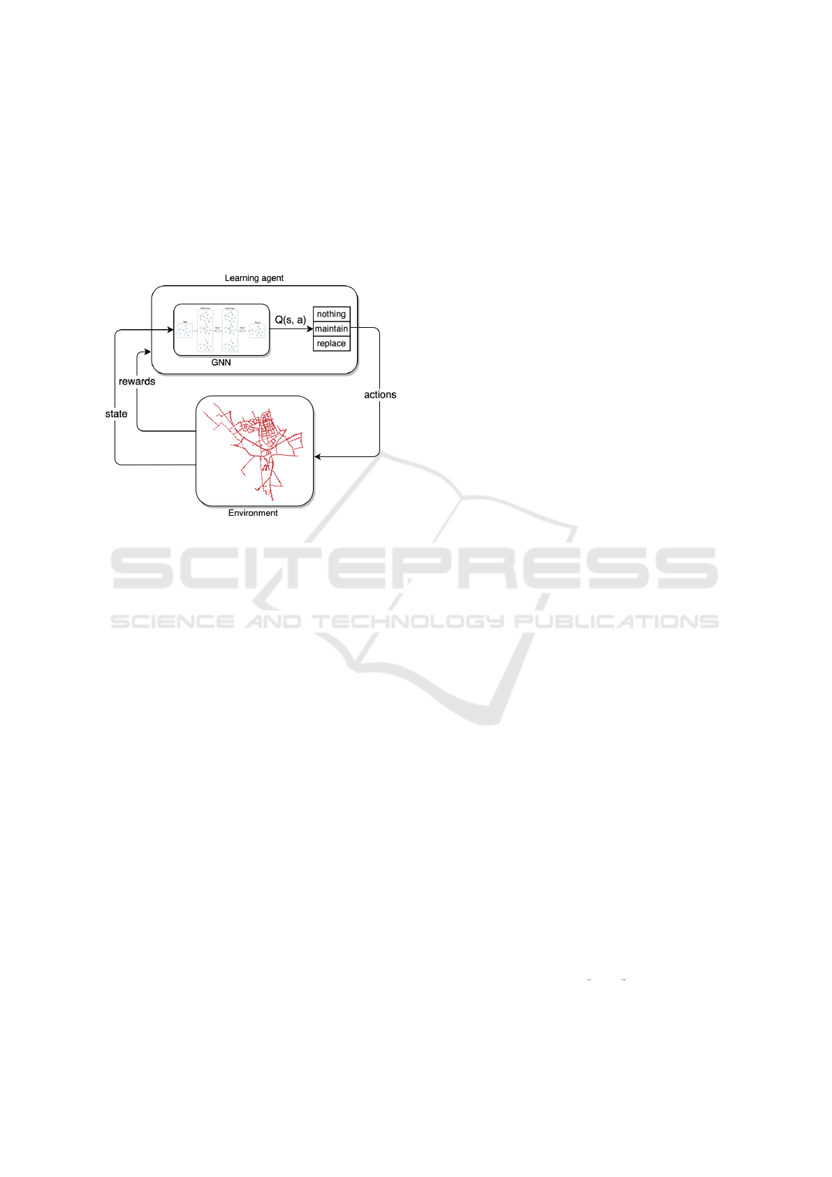
Figure 1: Interaction between DRL learning agent and en-
vironment, and the position of the GCN within the agent.
4 BACKGROUND
4.1 Deep Q Networks
Reinforcement learning algorithms aim at learning a
long-term strategy to maximize a cumulative reward.
An optimal strategy is learned by iteratively explor-
ing the state and action spaces, directed by the reward
function (Kaelbling et al., 1996). Q-learning (Watkins
and Dayan, 1992) is an RL algorithm that learns a pol-
icy π mapping states to actions. Every possible state-
action pair is stored in a table, and during training,
each entry is updated iteratively according to rewards
received. Rewards received in the future are geomet-
rically discounted using a discount factor γ ∈ [0, 1].
These values are called Q-values, and they represent
the expected cumulative discounted reward for exe-
cuting action a at state s and then following policy
π. Q-values are updated using the Bellman equation
defined below (Kaelbling et al., 1996):
Q(s,a) = R(s, a) + γmax
a
0
Q(s
0
,a
0
) (1)
where Q(s,a) is the Q-value function and R(s,a) the
reward function.
As problems become more complex with high-
dimensional state and action spaces, basic Q-learning
is not practical to use. Deep Q-Network (DQN) is
an algorithm proposed by (Mnih et al., 2013) based
on Q-learning that uses deep neural networks (DNN)
to estimate the Q-value function Q(s,a;θ) ≈ Q(s,a)
with parameters θ. This allows for leveraging the
generalization ability of DNN to estimate Q-values
for previously unseen state-action pairs. The DQN is
both a model-free and an off-policy algorithm (Mnih
et al., 2013). Due to the model-free feature, the con-
trol task is solved using samples obtained from the
simulated environment, without constructing an ex-
plicit model of the environment. With off-policy ap-
proach, the DQN follows a behaviour distribution and
ensures that the state space is adequately explored
while learning the greedy strategy a = max
a
Q(s,a; θ).
Practically, this means that an ε-greedy strategy is ap-
plied. The agent selects an action according to the
greedy strategy with probability 1 − ε, and selects a
random action with probability ε to provide a trade-
off between exploring new state-action pairs and ex-
ploiting the learned knowledge.
4.1.1 Double DQN
Double Deep Q-network (DDQN) is an improvement
on DQN proposed by van Hasselt et al. (2015). They
show that DQN sometimes suffers from overestima-
tions of Q-values. The computation of the target in the
optimization step of DQN includes a maximization
operator over estimated action values. Here, the same
value is used for selection and evaluation, making it
more likely to select overestimated values. DDQN
thus decouples action selection from evaluation. To
achieve this, DDQN evaluates the greedy policy with
an online Q-network, but it uses the target network for
estimating its value.
4.2 Graph Convolutional Networks
Graph Convolutional Network (GCN) is a neural net-
work model that directly encodes graph structure
(Kipf and Welling, 2017). The goal is to learn a func-
tion of features on a graph. It takes as input an m × n
feature matrix X consisting of feature vectors x
i
of
length n for each node i with 1 ≤ i ≤ m. It also takes
an adjacency matrix A describing the graph structure.
It produces a node-level output matrix with dimen-
sions m× o, where o is the number of output features.
The propagation function of GCN for layer l is:
f (H
(l)
,A) = σ
ˆ
D
−
1
2
ˆ
A
ˆ
D
−
1
2
H
(l)
W
(l)
(2)
Grouping of Maintenance Actions with Deep Reinforcement Learning and Graph Convolutional Networks
577

where
ˆ
A = I + A is the adjacency matrix with added
self-loops,
ˆ
D is the diagonal node degree matrix of
ˆ
A
and σ is a non-linear activation function.
5 METHODOLOGY AND
EMPIRICAL SETUP
5.1 Case Study: A Sewer Pipe Network
As a driver case for our work, we consider a real case
study of a network of sewer pipes. We choose a subset
of 942 pipes (assets) for evaluation of the DRL frame-
work. The available features for each pipe include
geographical location, material, length, and age. The
geographical location of the pipes is used to construct
the distance function described in Section 3. An ex-
ample in the context of our case study is given in the
following subsection. The resulting network serves
as input to the GCN. For deterioration modeling, we
utilize pipe failure rates extracted from a dataset of
26,285 manual pipe inspections. The inspections are
performed according to a standardized classification
scheme and provide damage observations of the in-
spected pipes. Every observed damage is assigned to
a class from 1 (minor damage) to 5 (worst damage).
The maintenance optimization problem can be
tackled in two ways. The first involves the model-
ing of deterioration of the assets under consideration
to estimate the failure behavior. The second consists
of finding the best moment for rehabilitation of assets,
given a deterioration model. In this work, we focus on
the latter. We employ a DRL framework with GNN
to plan rehabilitation activities, using a simple dete-
rioration model based on the exponential distribution
and failure rates obtained from historical data. Us-
ing a GNN to estimate failure rates and probabilities
is an exciting direction to explore in the future. This,
however, requires more extensive historical condition
monitoring data than is currently available.
We advocate investigating the capabilities of deep
reinforcement learning (DRL) in this setting. The
DRL agent follows the Double DQN algorithm (van
Hasselt et al., 2015; Mnih et al., 2013) and uses a
GNN to model the Q-value function. For this, we em-
ploy Graph Convolutional Networks (GCN) by Kipf
and Welling (2017). The DRL agent receives, at each
timestep, a representation of the sewer network’s state
from a simulated environment and uses the GCN to
select the next action to take based on this state (i.e.,
which pipes to maintain/replace). It then applies the
action to the environment and receives the next state
and a reward to evaluate the action taken. The inter-
action between the DRL agent and the environment is
depicted in Figure 1.
The transition dynamics are deterministic and
use the exponential distribution, which is commonly
used for modeling the lifespan of deteriorating assets
(Scheidegger et al., 2011; Birolini, 2013). There is
no uncertainty in our deterioration model because the
lifespan of underground sewer pipes is typically very
long, and they often are in use for an extended period
having a lifespan of 50 to 100 years (Petit-Boix et al.,
2016; Scheidegger et al., 2011). This is because sewer
pipes deteriorate slowly, resulting in a steady perfor-
mance for years. Therefore, it is highly unlikely that
failures occur in relatively newer pipes.
It is also important to note that we choose to use
a cost model with symbolic costs. This is because a
comprehensive cost model includes direct repair ex-
penses and indirect costs related to equipment and
labor costs. Additionally, performing maintenance
on pipe network results in additional social costs
due to service unavailability, traffic disruptions, dam-
aged properties in case of leakage, and health hazards
(Scheidegger et al., 2011). The monetization of such
indirect and social costs is complicated because they
are qualitative and not easily quantified. To monetize
all costs into a realistic cost model, dedicated valu-
ation methods are needed, often based on historical
maintenance data (Tscheikner-Gratl et al., 2019).
In the following, we explain how a graph is con-
structed from data and describe how the environment
simulates the sewer network by providing details of
states, actions, rewards, and transition dynamics.
5.2 Graph Representation
In order to apply a GCN to our specific case study
data, a graph representation is required. Let G =
(V,E) be a graph representing the sewer network
with nodes V and edges E. Let A be an adjacency
matrix with dimensions |V | × |V | where each entry
A
i j
∈ {0,1} denotes the absence or existence of an
edge between nodes i and j with 1 ≤ i, j ≤ |V |. Ev-
ery node v ∈ V corresponds to a sewer pipe, and ev-
ery edge e ∈ E represents a connection between two
pipes. The sewer network can be captured in a graph
in two ways. The first way resembles the real-world
pipe layout, such that there exists an edge between
two nodes only if the corresponding sewer pipes are
physically connected. The second way is based on a
distance measure. In this case, there exists an edge
between two nodes if their corresponding pipes are
within a given distance. We model the sewer network
based on the latter. For this, we define a distance mea-
sure by considering the distance between the coordi-
ICAART 2022 - 14th International Conference on Agents and Artificial Intelligence
578
nates of the start and end points of the pipes in the
physical world. Let dist(c
i
,c
j
) denote the distance in
meters between coordinates c
i
and c
j
and let c
s
i
and c
e
i
denote the coordinates corresponding to the start and
end points, respectively, of pipe i. Then the entries
of the adjacency matrix A are defined as follows, for
given distance r.
A
i j
=
1
i 6= j ∧ (dist(c
s
i
,c
s
j
) < r ∨
dist(c
s
i
,c
e
j
) < r ∨
dist(c
e
i
,c
s
j
) < r ∨
dist(c
e
i
,c
e
j
) < r)
0 otherwise
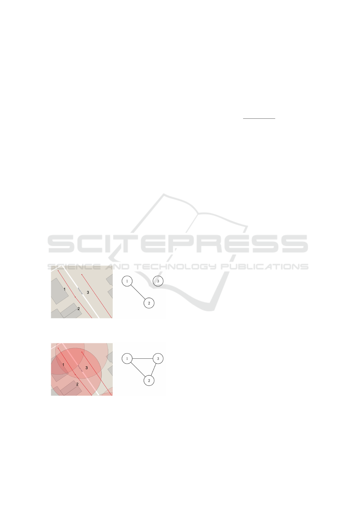
The sewer network graph representation of three spa-
tially close pipes are illustrated in Figure 2 based on
both, physical network and distance-based method.
5.3 Modeling of the Environment
5.3.1 Pipe Deterioration
To model the pipe deterioration mechanism, we use
a pipe-specific failure rate f r depending on the mate-
rial. We use damage observations from the inspection
records of the complete dataset to obtain these fail-
ure rates. We treat observations with damage class
4 or higher as a failure. We then count the num-
ber of failures per inspected pipe, divide them by the
(a) Graph based on physical pipe connections, where
nodes are only connected if their corresponding pipes
are connected in the real world.
(b) Graph with edges between nodes that have the start
or end points of their corresponding pipes within 20
meters distance of each other.
Figure 2: Two ways of representing the sewer pipes as
graph.
pipe length and average the result per material type
to obtain a failure rate per meter for each material
type. Let n f
i
denote the number of observed failures
of pipe i, I = {1, ...,N} a set of material types, and
B = {B
1
,..., B
N
} a set of pipes, where B
j
is a set of
pipes of material type j ∈ I. The failure rate m f r
j
of
material j is then obtained in the following way:
m f r
j
=
∑
i∈B
j
(n f
i
/l
i
)
|B
j
|
(3)
where l
i
is the length of pipe i. Finally, for each of
the 942 pipes under consideration, the pipe-specific
failure rate f r
i
is obtained by multiplying the failure
rate corresponding to the pipe material with the pipe’s
length.
The probability of failure p f is estimated using
the failure rates extracted from historical data and the
exponential distribution reliability function (Birolini,
2013) as follows:
p f
t
i
= 1 − rl
t
i
= 1 − e
− f r
i
aux
t
i
(4)
where p f
t
i
is the failure probability of pipe i at
timestep t, rl
t
i
the reliability level, f r
i
the failure rate
and aux
t
i
an auxiliary variable for the pipe age. An
auxiliary variable represents the physical condition of
the pipe, which can either improve or deteriorate de-
pending on the chosen actions. In summary, pipe de-
terioration depends on age, material, and length. The
deterioration model described above simplifies real-
ity to simulate the sewer network for the DRL agent.
More sophisticated ways of modeling deterioration
and extraction of failure rates from available data are
still an open problem.
5.3.2 States
Every node in the graph representing the pipe network
has a vector of features m
i
= hl
i
,w
i
,h
i
,mat
i
,age
i
,
f r
i
,aux
i
, p f
i
,rl
i
i, with 1 ≤ i ≤ m (m being total num-
ber of nodes) and where l
i
is the length, w
i
and h
i
are
the diameter width and height of the pipe, mat
i
is the
material, age
i
is the age, f r
i
is the failure rate, aux
i
is an auxiliary variable for the age that represents the
change in physical state of the pipe, p f
i
is the proba-
bility of failure and rl
i
is the reliability. On each step
aux
i
, rl
i
and p f
i
are updated depending on the action
applied. The age
i
is incremented to reflect the actual
age and does not depend on applied actions to avoid
modifications to the original age values of the pipes.
All feature vectors form a feature matrix with dimen-
sions m ×n representing the environment state, where
n is the number of features. In addition, there is an ad-
jacency matrix A = m × m representing a set of edges
connecting the nodes.
Grouping of Maintenance Actions with Deep Reinforcement Learning and Graph Convolutional Networks
579

5.3.3 Actions
At each time step t the DRL agent selects the best ac-
tion for each pipe given the current state, resulting in
a vector a = ha
t
1
,a
t
2
,..., a
t
m
i. The set of actions con-
sists of three types, such that at each timestep t for
each pipe i, an agent can choose a
t
i
∈ {0,1, 2}. Action
0 means do nothing, action 1 is maintain, and action
2 is replace.
5.3.4 Reward Function
The reward function R(s
t
,a
t
) provides the immediate
reward for taking actions a
t
from state s
t
. Since the
total cost should be minimized, we inverse the reward
function. As described, in each timestep t an action
is applied to every pipe i. This results in a reward
vector r
t
= hr
t
1
+ b
t
1
,..., r
t
m
+ b
t
m
i where each r
t
i
and b
t
i
are obtained in the following way:
r
t
i
=
0 if a
t
i
= do
nothing and p f
t
i
< 0.9
−1 if a
t
i
= do nothing and p f
t
i
≥ 0.9
−0.5 if a
t
i
= maintain and p f
t
i
> 0.5
−1 if a
t
i
= maintain and p f
t
i
≤ 0.5
−0.8 if a
t
i
= replace and p f
t
i
> 0.5
−1 if a
t
i
= replace and p f
t
i
≤ 0.5
b
t
i
=
(
0.1 if a
t
i
6= 0 ∧ ∃ j, j 6= i ∧ A
i j
= 1 ∧ a
t
j
6= 0
0 otherwise
A penalty of −1 is introduced to discourage the
agent from selecting maintenance or replacement ac-
tions for pipes that are in good shape. The same
penalty helps to ensure a sufficient reliability level if
a pipe has a high probability of failure, but the agent
chooses to do nothing. Practically, these penalty val-
ues relate to the impact on traffic, surroundings, and
network unavailability in case of pipe failures.
In addition, grouped rehabilitation is rewarded. If
for a certain pipe i the maintain or replace action is
selected, while one of these actions is also selected
for any neighbor j of pipe i (i.e. there is an edge con-
necting i and j), then both pipes i and j receive a small
bonus (or cost reduction) of 0.1, denoted above by b
i
.
These bonus values are concerned with cost reduction
due to one-time setup and transportation costs if pipes
in closed proximity are maintained together.
5.3.5 Transitions
When actions are applied to the network, the environ-
ment moves ahead one timestep and produces a new
state representation and a reward. The state represen-
tation consists of a new matrix of pipe features. The
adjacency matrix remains the same since the layout
of the sewer network is fixed. Because the environ-
ment is modeled as MDP, the next state is only de-
pendent on the previous state and action. For the next
timestep, the age feature age
t+1
i
is increased by one
year, and the auxiliary feature aux
t+1
i
describing the
physical state of pipe i is computed as follows:
aux
t+1
i
=
aux
t
i
+ 1 if a
t
i
= do nothing
aux
t
i
− 10 if a
t
i
= maintain and
aux
t
i
> 10
aux
t
i
if a
t
i
= maintain and
aux
t
i
≤ 10
1 if a
t
i
= replace
So if do nothing is applied to a pipe, the auxiliary
feature increases by 1 year, if maintain is applied, it
decreases by 10 years and if replace is applied, it is
reset to 1. Based on this auxiliary age feature, the
new failure probability and reliability are computed
for every pipe using the exponential distribution given
in equation 4.
6 EVALUATION AND RESULTS
6.1 Implementation
We implement the DRL framework with DDQN in
Python. The environment is a custom OpenAI Gym
environment. For the neural network architecture
with GCN, we use PyTorch Geometric (Fey and
Lenssen, 2019).
The network takes a 942 × 11 node feature matrix
as input for 942 pipes with 9 features. The material
is represented using one-hot encoding. The dataset
has 3 material types, resulting in 3 material columns
(hence the input shape). Besides the node features,
the network takes the adjacency matrix describing the
edge connections. The network architecture consists
of two GCNConv layers with an output size of 32, each
followed by a ReLU activation function. The final
layer is a fully connected Linear with output size 3
(# actions). For network optimization, AdamW is used
with MSELoss.
We compare DRL with GCN (referred to as
DRL+GCN) to several baselines to show the potential
of applying GCN in a DRL framework. First, we ap-
ply the same DRL framework, but the GCN architec-
ture is replaced for a simple, fully connected Linear
layer with the same input and output size (referred to
ICAART 2022 - 14th International Conference on Agents and Artificial Intelligence
580
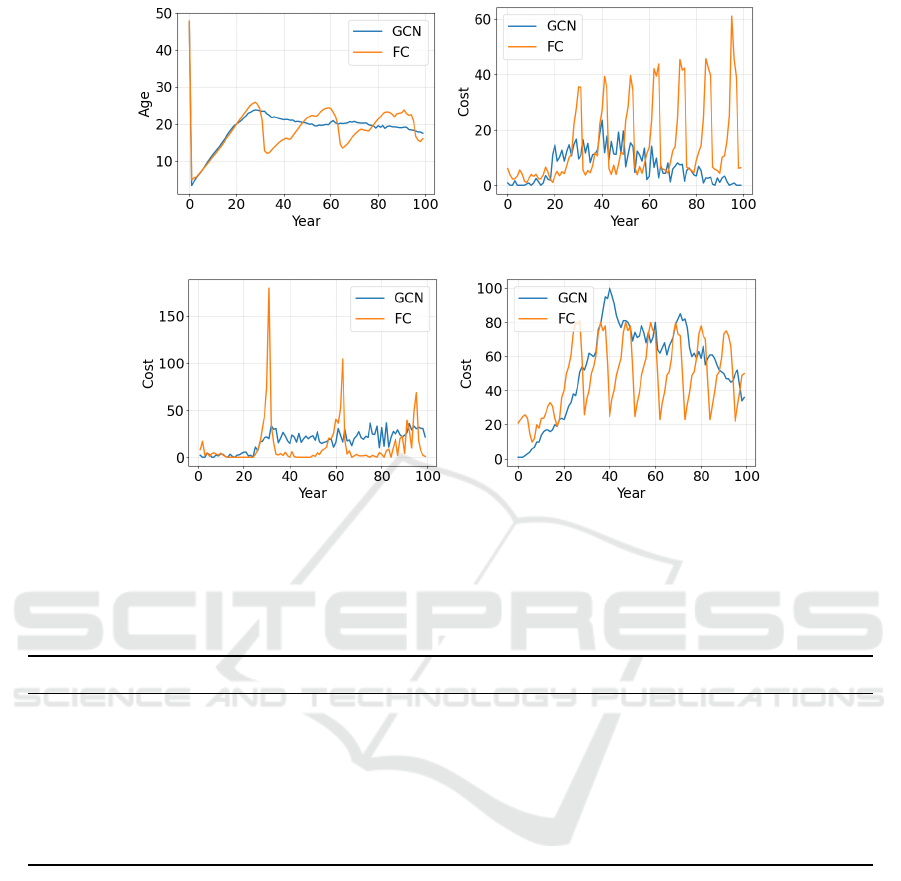
(a) Mean pipe age per year. (b) Maintenance costs per year.
(c) Replacement costs per year, excluding
1st.
(d) ‘Do nothing’ penalties per year.
Figure 3: Breakdown of the total costs per year of each action type for DRL+GCN and DRL+FC. The top left diagram shows
the mean pipe age, which is influenced by intervention actions.
Table 1: Comparison of DRL+GCN with DRL having fully connected layers, two preventive and one corrective baselines.
DRL+GCN DRL+FC Replace Greedy Maintain-10
Mean # pipes per group 2.74 2.02 - - -
% groups with >1 pipe 56% 30% - - -
Mean reliability 0.46 0.42 0.32 0.56 0.15
Interventions per year 45.26 55.94 20.77 378.45 94.2
Interventions per pipe 4.80 5.94 2.44 40.18 10
Total cost based on reward function 8362 8077 21,769 15,526 50,908
as DRL+FC). We also compare with non-RL strate-
gies traditionally applied in industry (Ahmad and Ka-
maruddin, 2012), including time-based preventive,
greedy preventive, and corrective approaches. The
time-based approach suggests maintain action for all
pipes based on a time interval of 10 years. The
greedy preventive approach chooses maintain action
as cheapest intervention as soon as the p f
i
> 0.5. In
the corrective approach, interventions are taken after
failure, represented as p f
i
> 0.95. The rationale be-
hind choosing a threshold of 0.95, instead of 0.9 as in
the reward function, is, because in the corrective ap-
proach, pipes are only replaced after they have already
failed. We use the same simulated environment, in-
cluding reward functions, penalties, and bonus costs,
for all three baselines for fair comparison. This re-
sults in two preventive strategies, i.e, Maintain-10 and
Greedy, and one corrective strategy, i.e, Replace.
6.2 Training
A graph is constructed from the pipes in the dataset,
which consists of two coordinate points. A node rep-
resents a pipe, and an edge exists between two pipes
if any of their points are within a range of 20 meters
of each other. We train the network using a Google
Colab notebook with GPU for 6000 episodes of 100
timesteps with a replay memory size of 500. The net-
work weights are updated by selecting random sam-
ples from replay memory with a batch size of 32 and
computing the expected accumulated discounted re-
ward with discount factor γ = 0.9. The DRL agent
Grouping of Maintenance Actions with Deep Reinforcement Learning and Graph Convolutional Networks
581
follows an ε-greedy strategy with ε annealed linearly
from 1 to 0.01, and the learning rate of the optimizer
is set to 1 × 10
−4
.
6.3 Results
After training, we generate maintenance plans for
a planning horizon of 100 years for all 942 pipes.
For the first year, the DRL+GCN maintenance plan
proposes to replace most of the pipes because ini-
tially, the average pipe age is 48 years, causing low-
reliability levels. This is because the probability of
failure of pipes is based on failure rates and the cur-
rent age of the pipe. When most pipes are replaced,
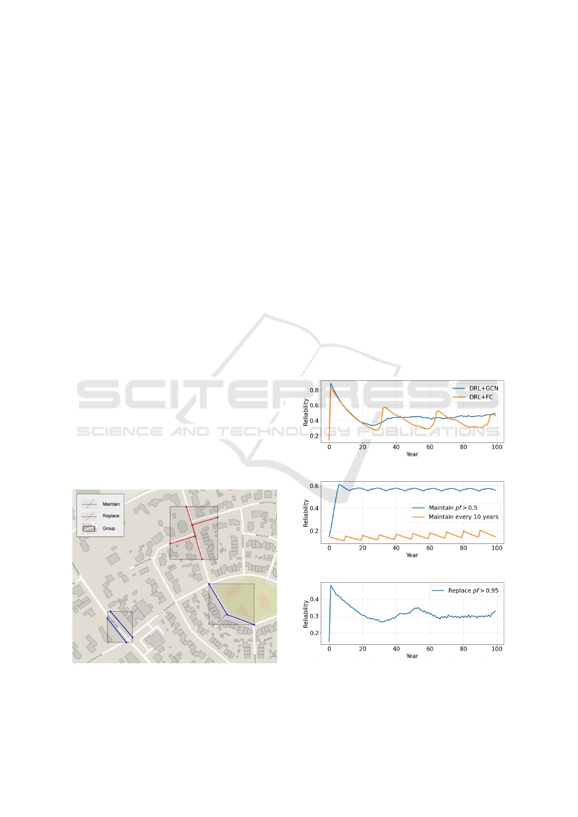
the reliability becomes very high, as can be seen by a
peak in Figure 5a. Then, as the reliability decreases
over the years, the number of rehabilitation actions
starts to increase, resulting in higher yearly costs, as
shown in Figure 6a. Also, note that the DRL+GCN
agent suggests frequent interventions in a planning
horizon resulting in a steady reliability level and to-
tal intervention costs, as can be noted in Figure 3.
One of the key goals to employ GCN with DRL
is to achieve intervention grouping to optimize main-
tenance plans. A group is defined as a set of pipes
such that edges connect the corresponding nodes in
the graph. The higher the number of pipes per group,
the more rehabilitation activities are concentrated in
a smaller amount of different geographical locations,
resulting in less setup and transportation costs as
shown in (Rokstad and Ugarelli, 2015; Pargar et al.,
2017). The GCN creates a plan in which 56% of
the groups have more than one pipe, resulting in an
average of 2.74 pipes per group across 100 years
(see Table 1). An example of grouping produced by
Figure 4: Example of a grouping of interventions on pipes
that are close to each other, produced by the DRL+GCN
approach for year 50 of the maintenance plan.
the DRL+GCN approach is shown in Figure 4. We
present a comparison with baselines in the following
section.
6.4 Baseline Comparison
We compare the proposed DRL+GCN approach with
four other baselines. Table 1 provides the compari-
son of all the considered approaches. The costs dis-
played are the values produced by the reward func-
tion. This includes the costs of the actions themselves,
bonus values for grouped rehabilitation, and penal-
ties for both unnecessary interventions and poor re-
liability while no intervention is suggested. The strat-
egy with the lowest cost while maintaining an ade-
quate reliability level is preferred. The greedy ap-
proach shows the highest average reliability, but it is
also significantly more expensive than the two DRL-
based strategies. Maintain-10 does not perform well
in terms of both cost and reliability. The corrective ap-
proach (Replace) gives relatively low reliability while
also incurring high costs. Although the replace strat-
egy shows the least number of interventions, the over-
all reliability of the network is also low because pipes
deteriorate until they fail, incurring higher costs.
(a) DRL approach.
(b) Preventive approach.
(c) Corrective approach.
Figure 5: Mean reliability per year for each strategy.
ICAART 2022 - 14th International Conference on Agents and Artificial Intelligence
582
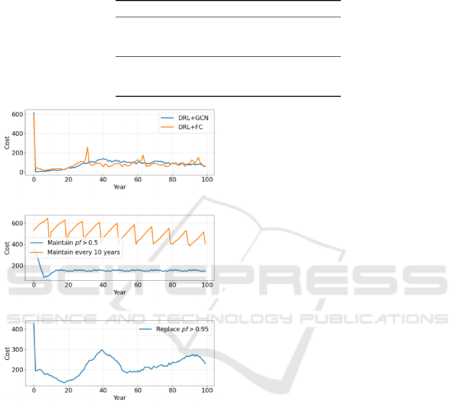
Table 2: Breakdown of total costs of each action for the DRL approaches with GCN and fully-connected (FC) layer over
100 years, as computed with the reward function. The highest costs are caused by doing nothing, incurring penalties for low
reliability levels. Without the penalties, the GCN approach performs significantly better than the FC method.
GCN FC
Cost of maintenance actions 683.6 1451.2
Cost of replacement actions 2332.4 1752.3
Cost of do nothing actions/penalties 5346.0 4873.0
Total cost based on reward function 8362.0 8076.5
Total without action ‘nothing’ penalties 3016.0 3203.5
Total without any penalties or bonus 3196.0 3491.8
(a) DRL approach.
(b) Preventive approach.
(c) Corrective approach.
Figure 6: Total cost per year for each strategy, as computed
by the reward function.
We provide a detailed comparison of DRL+GCN
and DRL+FC approaches. The GCN favors replace-
ment actions, while FC prefers maintenance. Figure
3 shows the costs per year of each action according
to the reward function. The FC chooses actions ac-
cording to a recurring pattern where the pipes age and
deteriorate to the point that the reliability becomes too
low, triggering many interventions simultaneously. In
contrast, the GCN approach spreads the interventions
more realistically over the years, resulting in a more
stable reliability level and fewer yearly cost fluctua-
tions compared to the FC plan. This is also aligned
with real budgeting of infrastructure agencies where
a limited budget is available for rehabilitation activi-
ties each year (Rokstad and Ugarelli, 2015; Li et al.,
2011). Stable annual costs are therefore desirable.
A maintenance plan with fluctuating costs that cause
the budget to be only partially utilized in some years,
while causing a deficit in other years, would be ineffi-
cient and unsuitable in practice. Furthermore, the FC
approach is likely to pose an additional risk of pipe
failure since the pipes deteriorate for a extended pe-
riod before any action is suggested. In the current
configuration, the GCN approach is more expensive
mainly because of the ‘do nothing’-actions, which in-
cur penalties for pipes with low reliability. Figure 3d
shows that for GCN, these yearly penalties get to a
peak and then gradually decrease. For the FC plan,
however, the same pattern keeps repeating without
improvement. When only the costs for maintenance
and replacement without penalties are taken into ac-
count, the GCN is less expensive, as shown in table
2.
Figure 5 and 6 provide an overview of averaged
reliability and cost per year for the complete plan-
ning horizon. It is noted that the greedy approach
shows overall high reliability, but it is substantially
more expensive compared to other approaches. Our
DRL+GCN approach is second in terms of aver-
aged reliability and costs. Besides, we also com-
pare metrics related to the grouping of intervention
actions for the DRL approaches. Taking all metrics
from Table 1 into account, we see that although the
DRL+GCN strategy is slightly more expensive than
the simpler variant DRL+FC, it provides better relia-
bility, a higher degree of grouping, and fewer number
of interventions.
7 CONCLUSIONS AND FUTURE
WORK
This work presents a deep reinforcement learning
framework that combines DDQN and GCN for the re-
Grouping of Maintenance Actions with Deep Reinforcement Learning and Graph Convolutional Networks
583

habilitation planning of sewer pipes. The DRL agent
learns an improved policy in terms of lower cost and
higher reliability and uses GCN to leverage the rela-
tional information encoded in the graph structure of
the sewer network. Our framework is successfully
evaluated on a real dataset to show its potential for
applications in infrastructure maintenance planning.
The proposed approach is network and environment
agnostic, is not intended to solve the specific case
study described in this paper but to serve as a feasi-
bility study for applying the combination of deep rein-
forcement learning with graph neural networks for as-
set management problems. Different neural network
architectures can be plugged in, and the environment
can be easily modified with specific problem settings.
An asset deterioration model that more accurately
resembles reality remains an open problem for the fu-
ture. This includes a more sophisticated way of ex-
tracting/predicting fail rates and the use of additional
data sources to include geographic and demographic
data of the surrounding area, such as traffic load, tree
density, and soil information of assets network. An-
other future problem is a reward function that better
accounts for different costs (e.g., replacement cost,
failure cost, unavailability costs) and asset-specific
aspects (e.g., material, length, impact on surrounding
infrastructure).
ACKNOWLEDGEMENTS
This research has been partially funded by NWO un-
der the grant PrimaVera NWA.1160.18.238.
REFERENCES
Ahmad, R. and Kamaruddin, S. (2012). An overview of
time-based and condition-based maintenance in in-
dustrial application. Computers & Industrial Engi-
neering, 63(1):135–149.
Almasan, P., Su
´
arez-Varela, J., Badia-Sampera, A., Rusek,
K., Barlet-Ros, P., and Cabellos-Aparicio, A. (2020).
Deep Reinforcement Learning meets Graph Neural
Networks: exploring a routing optimization use case.
arXiv:1910.07421 [cs]. arXiv: 1910.07421.
Battaglia, P. W., Hamrick, J. B., Bapst, V., Sanchez-
Gonzalez, A., Zambaldi, V., Malinowski, M., Tac-
chetti, A., Raposo, D., Santoro, A., Faulkner, R., Gul-
cehre, C., Song, F., Ballard, A., Gilmer, J., Dahl, G.,
Vaswani, A., Allen, K., Nash, C., Langston, V., Dyer,
C., Heess, N., Wierstra, D., Kohli, P., Botvinick, M.,
Vinyals, O., Li, Y., and Pascanu, R. (2018). Relational
inductive biases, deep learning, and graph networks.
Birolini, A. (2013). Reliability engineering: theory and
practice. Springer Science & Business Media.
Chen, Y. F., Everett, M., Liu, M., and How, J. P. (2017). So-
cially aware motion planning with deep reinforcement
learning. In 2017 IEEE/RSJ International Confer-
ence on Intelligent Robots and Systems (IROS), pages
1343–1350.
da Costa, P. R., Rhuggenaath, J., Zhang, Y., and Akcay,
A. (2020). Learning 2-opt heuristics for the traveling
salesman problem via deep reinforcement learning. In
Asian Conference on Machine Learning, pages 465–
480. PMLR.
Dai, H., Khalil, E. B., Zhang, Y., Dilkina, B., and Song,
L. (2018). Learning combinatorial optimization algo-
rithms over graphs.
Fey, M. and Lenssen, J. E. (2019). Fast graph represen-
tation learning with PyTorch Geometric. In ICLR
Workshop on Representation Learning on Graphs and
Manifolds.
Fontecha, J. E., Agarwal, P., Torres, M. N., Mukherjee,
S., Walteros, J. L., and Rodr
˜
Aguez, J. P. (2021). A
two-stage data-driven spatiotemporal analysis to pre-
dict failure risk of urban sewer systems leveraging ma-
chine learning algorithms. Risk Analysis.
Garg, S., Bajpai, A., and Mausam (2019). Size Independent
Neural Transfer for RDDL Planning. Proceedings of
the International Conference on Automated Planning
and Scheduling, 29:631–636.
Hansen, B. D., Jensen, D. G., Rasmussen, S. H., Tamouk,
J., Uggerby, M., and Moeslund, T. B. (2019). General
Sewer Deterioration Model Using Random Forest. In
2019 IEEE Symposium Series on Computational In-
telligence (SSCI), pages 834–841.
Hu, L., Liu, Z., Hu, W., Wang, Y., Tan, J., and Wu,
F. (2020). Petri-net-based dynamic scheduling of
flexible manufacturing system via deep reinforcement
learning with graph convolutional network. Journal of
Manufacturing Systems, 55:1–14.
Janisch, J., Pevn
´
y, T., and Lis
´
y, V. (2021). Symbolic Rela-
tional Deep Reinforcement Learning based on Graph
Neural Networks. arXiv:2009.12462 [cs]. arXiv:
2009.12462.
Joshi, C. K., Laurent, T., and Bresson, X. (2019). An ef-
ficient graph convolutional network technique for the
travelling salesman problem.
Kaelbling, L. P., Littman, M. L., and Moore, A. W. (1996).
Reinforcement Learning: A Survey. Journal of Artifi-
cial Intelligence Research, 4:237–285.
Kipf, T. N. and Welling, M. (2017). Semi-supervised clas-
sification with graph convolutional networks.
Li, F., Sun, Y., Ma, L., and Mathew, J. (2011). A grouping
model for distributed pipeline assets maintenance de-
cision. In 2011 International Conference on Quality,
Reliability, Risk, Maintenance, and Safety Engineer-
ing, pages 601–606.
Li, Y. (2017). Deep reinforcement learning: An overview.
arXiv preprint arXiv:1701.07274.
Luong, N. C., Hoang, D. T., Gong, S., Niyato, D., Wang,
P., Liang, Y.-C., and Kim, D. I. (2019). Applica-
tions of Deep Reinforcement Learning in Communi-
cations and Networking: A Survey. IEEE Communi-
cations Surveys Tutorials, 21(4):3133–3174. Confer-
ICAART 2022 - 14th International Conference on Agents and Artificial Intelligence
584

ence Name: IEEE Communications Surveys Tutori-
als.
Mnih, V., Badia, A. P., Mirza, M., Graves, A., Lillicrap,
T. P., Harley, T., Silver, D., and Kavukcuoglu, K.
(2016). Asynchronous methods for deep reinforce-
ment learning.
Mnih, V., Kavukcuoglu, K., Silver, D., Graves, A.,
Antonoglou, I., Wierstra, D., and Riedmiller, M.
(2013). Playing atari with deep reinforcement learn-
ing.
Pargar, F., Kauppila, O., and Kujala, J. (2017). Inte-
grated scheduling of preventive maintenance and re-
newal projects for multi-unit systems with grouping
and balancing. Computers & Industrial Engineering,
110:43–58.
Petit-Boix, A., Roig
´
e, N., de la Fuente, A., Pujadas, P.,
Gabarrell, X., Rieradevall, J., and Josa, A. (2016). In-
tegrated structural analysis and life cycle assessment
of equivalent trench-pipe systems for sewerage. Wa-
ter Resources Management, 30(3):1117–1130.
Prates, M., Avelar, P. H. C., Lemos, H., Lamb, L. C., and
Vardi, M. Y. (2019). Learning to Solve NP-Complete
Problems: A Graph Neural Network for Decision
TSP. Proceedings of the AAAI Conference on Arti-
ficial Intelligence, 33(01):4731–4738. Number: 01.
Puterman, M. L. (1994). Markov Decision Processes: Dis-
crete Stochastic Dynamic Programming. Wiley Series
in Probability and Statistics. Wiley.
Rokstad, M. M. and Ugarelli, R. M. (2015). Minimising the
total cost of renewal and risk of water infrastructure
assets by grouping renewal interventions. Reliability
Engineering & System Safety, 142:148–160.
Scheidegger, A., Hug, T., Rieckermann, J., and Maurer,
M. (2011). Network condition simulator for bench-
marking sewer deterioration models. Water Research,
45(16):4983–4994.
Sun, P., Lan, J., Li, J., Guo, Z., and Hu, Y. (2021). Combin-
ing Deep Reinforcement Learning With Graph Neu-
ral Networks for Optimal VNF Placement. IEEE
Communications Letters, 25(1):176–180. Conference
Name: IEEE Communications Letters.
Sutton, R. S., McAllester, D., Singh, S., and Mansour, Y.
(1999). Policy gradient methods for reinforcement
learning with function approximation. NIPS’99, page
1057–1063, Cambridge, MA, USA. MIT Press.
Tesauro, G. (1995). Temporal difference learning and td-
gammon. Commun. ACM, 38(3):58–68.
Tscheikner-Gratl, F., Caradot, N., Cherqui, F., Leit
˜
ao, J. P.,
Ahmadi, M., Langeveld, J. G., Gat, Y. L., Scholten,
L., Roghani, B., Rodr
´
ıguez, J. P., Lepot, M., Stege-
man, B., Heinrichsen, A., Kropp, I., Kerres, K.,
do C
´
eu Almeida, M., Bach, P. M., de Vitry, M. M.,
Marques, A. S., Sim
˜
oes, N. E., Rouault, P., Her-
nandez, N., Torres, A., Werey, C., Rulleau, B., and
Clemens, F. (2019). Sewer asset management – state
of the art and research needs. Urban Water Journal,
16(9):662–675.
van Hasselt, H., Guez, A., and Silver, D. (2015). Deep re-
inforcement learning with double q-learning.
Veli
ˇ
ckovi
´
c, P., Cucurull, G., Casanova, A., Romero, A., Li
`
o,
P., and Bengio, Y. (2018). Graph attention networks.
Watkins, C. J. C. H. and Dayan, P. (1992). Q-learning. Ma-
chine Learning, 8(3):279–292.
Weeraddana, D., Liang, B., Li, Z., Wang, Y., Chen, F.,
Bonazzi, L., Phillips, D., and Saxena, N. (2020). Uti-
lizing machine learning to prevent water main breaks
by understanding pipeline failure drivers.
Yan, Z., Ge, J., Wu, Y., Li, L., and Li, T. (2020). Automatic
Virtual Network Embedding: A Deep Reinforcement
Learning Approach With Graph Convolutional Net-
works. IEEE Journal on Selected Areas in Communi-
cations, 38(6):1040–1057. Conference Name: IEEE
Journal on Selected Areas in Communications.
Yin, X., Chen, Y., Bouferguene, A., and Al-Hussein, M.
(2020). Data-driven bi-level sewer pipe deterioration
model: Design and analysis. Automation in Construc-
tion, 116:103181.
Grouping of Maintenance Actions with Deep Reinforcement Learning and Graph Convolutional Networks
585
