
Evaluation of RGB and LiDAR Combination for Robust Place
Recognition
Farid Alijani
1 a
, Jukka Peltom
¨
aki
1 b
, Jussi Puura
2
, Heikki Huttunen
3 c
,
Joni-Kristian K
¨
am
¨
ar
¨
ainen
1 d
and Esa Rahtu
1 e
1
Tampere University, Finland
2
Sandvik Mining and Construction Ltd, Finland
3
Visy Oy, Finland
Keywords:
Visual Place Recognition, Image Retrieval, Deep Convolutional Neural Network, Deep Learning for Visual
Understanding.
Abstract:
Place recognition is one of the main challenges in localization, mapping and navigation tasks of self-driving
vehicles under various perceptual conditions, including appearance and viewpoint variations. In this paper,
we provide a comprehensive study on the utility of fine-tuned Deep Convolutional Neural Network (DCNN)
with three MAC, SpoC and GeM pooling layers to learn global image representation for place recognition in
an end-to-end manner using three different sensor data modalities: (1) only RGB images; (2) only intensity
or only depth 3D LiDAR point clouds projected into 2D images and (3) early fusion of RGB images and
LiDAR point clouds (both intensity and depth) to form a unified global descriptor to leverage robust features
of both modalities. The experimental results on a diverse and large long-term Oxford Radar RobotCar dataset
illustrate an achievement of 5 m outdoor place recognition accuracy with high recall rate of 90 % using early
fusion of RGB and LiDAR sensor data modalities when fine-tuned network with GeM pooling layer is utilized.
1 INTRODUCTION
Place recognition is a fundamental component in
the long-term navigation stack of the robotic sys-
tems in real-world applications, ranging from au-
tonomous vehicles to drones and computer vision sys-
tems (Lowry et al., 2016). Used for variety of appli-
cations such as localization, image retrieval and loop
closure detection in GPS denied environments, it is
the process of recognizing a previously visited place
using visual content, often under varying appearance
conditions and viewpoint changes with certain com-
putational constraints.
A common practice to obtain a precise location of
an agent in an unknown environment is to first collect
a database of images with different sensor modalities
such as camera or LiDAR, stamped with their pre-
cise GNSS/INS or odometry positions. Then given a
a
https://orcid.org/0000-0003-3928-7291
b
https://orcid.org/0000-0002-9779-6804
c
https://orcid.org/0000-0002-6571-0797
d
https://orcid.org/0000-0002-5801-4371
e
https://orcid.org/0000-0001-8767-0864
query image or LiDAR scan of a place, we search the
stored database to retrieve the best match which re-
veals the exact pose of that query with respect to the
reference database (gallery).
Robust and efficient feature representation meth-
ods with powerful discriminatory performance are
crucial to solve the place recognition task. These
can mainly be categorized as image-based and point
cloud-based approaches (Liu et al., 2019). Compared
to the conventional approaches (Cummins and New-
man, 2008; Milford and Wyeth, 2012) and the deep
learning approaches (Arandjelovic et al., 2018) ap-
plied to RGB images, learning local or global repre-
sentations of raw LiDAR point clouds for place recog-
nition is very challenging and still an open research
question (Zou et al., 2019) due to its irregular un-
ordered structure and lack of robust descriptors.
Although raw LiDAR point clouds suffer from
lacking the detailed texture information compared to
RGB images and similar corner or edge features may
easily lead to false positives in the LiDAR-based
place recognition, the availability of precise depth
information enables more accurate place recognition
using LiDAR point clouds compared to RGB images.
650
Alijani, F., Peltomäki, J., Puura, J., Huttunen, H., Kämäräinen, J. and Rahtu, E.
Evaluation of RGB and LiDAR Combination for Robust Place Recognition.
DOI: 10.5220/0010909100003124
In Proceedings of the 17th International Joint Conference on Computer Vision, Imaging and Computer Graphics Theory and Applications (VISIGRAPP 2022) - Volume 5: VISAPP, pages
650-658
ISBN: 978-989-758-555-5; ISSN: 2184-4321
Copyright
c
2022 by SCITEPRESS – Science and Technology Publications, Lda. All rights reserved

Furthermore, the geometric information of the Li-
DAR point clouds is invariant to enormous illumina-
tion changes which leads to more robust place recog-
nition over different times, days and seasons in an en-
tire year.
Following (Shi et al., 2015; Su et al., 2015), we
project 3D LiDAR point clouds into 2D images and
apply 2-dimensional DCNN to obtain an improved
global feature retrieval performance. In this paper,
our contribution is to provide a comprehensive study
on the utility of the fine-tuned DCNNs with three
MAC, SpoC and GeM pooling layers to learn global
image representations for place recognition in an end-
to-end manner for three different sensor data modali-
ties: (1) only RGB images; (2) only intensity or depth
3D point clouds projected into 2D images and (3)
early fusion of RGB images and LiDAR point clouds
(both intensity and depth) to form a unified global de-
scriptor to leverage robust features of both modalities.
The rest of this paper is organized as follows. Sec-
tion 2 briefly discusses the related work. In section 3,
we provide the baseline method along with section 4
which explains the real-world outdoor datasets to ad-
dress the visual place recognition task. In section 5,
we show the experimental results and conclude the
paper in section 6.
2 RELATED WORK
Image-based Place Recognition. One of the most
crucial parts of a place recognition system is the im-
age representation, similar to the most visual recog-
nition tasks, including image retrieval, image clas-
sification and object detection (Lowry et al., 2016;
Zhang et al., 2021). Conventional methods extract
handcrafted local invariant features (Lowe, 2004; Bay
et al., 2008) and aggregate them into global descrip-
tors (Filliat, 2007; J
´
egou et al., 2010; J
´
egou et al.,
2010; Torii et al., 2015) as image representation.
The main problem with traditional handcrafted fea-
tures is that they are not robust enough with respect
to the environmental variations such as lighting con-
ditions, scales and viewpoints (Masone and Caputo,
2021). With the rise of deep learning methods, DC-
NNs outperformed conventional approaches to learn
deep and compact visual representation (Radenovi
´
c
et al., 2016; Radenovi
´
c et al., 2018; Radenovi
´
c et al.,
2019; Kalantidis et al., 2016; Tolias et al., 2016b;
Arandjelovic et al., 2018).
Pointcloud-based Place Recognition. LiDAR-based
place recognition has become a compelling research
topic, over the past few years, thanks to its irre-
placeable data structure. It contains informative 3D
structural information of the environment and is more
robust against illumination and seasonal variations.
Compared to RGBD cameras, laser sensors provide
longer working range which makes them suitable, es-
pecially, for perception of outdoor scenes. Few of
the recent work which concentrated on learning deep
descriptors of 3D point clouds are (He et al., 2016;
Dewan et al., 2018; Klokov and Lempitsky, 2017).
Dub
´
e et al. (Dub
´
e et al., 2017) propose SegMatch as a
technique for enabling autonomous vehicles to recog-
nize previously visited areas based on the extraction
and matching of 3D segments of LiDAR point clouds.
SegMatch can recognize places at object-level even
though there is no intact object.
Uy and Lee (Uy and Lee, 2018) integrate Point-
Net (Charles et al., 2017) and NetVLAD (Arand-
jelovic et al., 2018), to obtain PointNetVLAD in order
to tackle place recognition in large-scale scenes. It
extracts discriminative global representations of raw
LiDAR data. The authors formulate place recognition
as a metric learning problem and present a lazy triplet
and quadruplet loss function to train the proposed
network end-to-end. It, however, does not consider
the local structure information and ignores the spa-
tial distribution of local features. PCAN (Zhang and
Xiao, 2019) improves PointNetVLAD by learning an
attention map for aggregation, using an architecture
inspired by PointNet++ (Qi et al., 2017). Liu et
al. (Liu et al., 2019) present LPD-Net to learn global
descriptors from 3D point clouds. Compared with
PointNetVLAD (Uy and Lee, 2018), LPD-Net con-
siders the spatial distribution of similar local struc-
tures, which is capable of improving the recognition
performance and gaining more robustness with re-
spect to weather or illumination changes.
Compared to the image-based place recognition,
the LiDAR-based approaches are still growing. Al-
though handcrafted 3D descriptors have been used for
recognition tasks (Rusu et al., 2009), using classical
global pooling techniques such as GeM (Radenovi
´
c
et al., 2019) pooling layer applied to LiDAR-based or
image-LiDAR-based approaches is still relatively un-
touched (Martinez et al., 2020).
3 PROCESSING PIPELINE
In this work, we concentrate on the deep image repre-
sentation obtained by DCNN in which given an input
an image, it produces a global descriptor to describe
the visual content of the image. For training, Raden-
ovic et al. (Radenovi
´
c et al., 2019) adopt the Siamese
neural network architecture. The Siamese architec-
ture is trained using positive and negative image pairs
Evaluation of RGB and LiDAR Combination for Robust Place Recognition
651
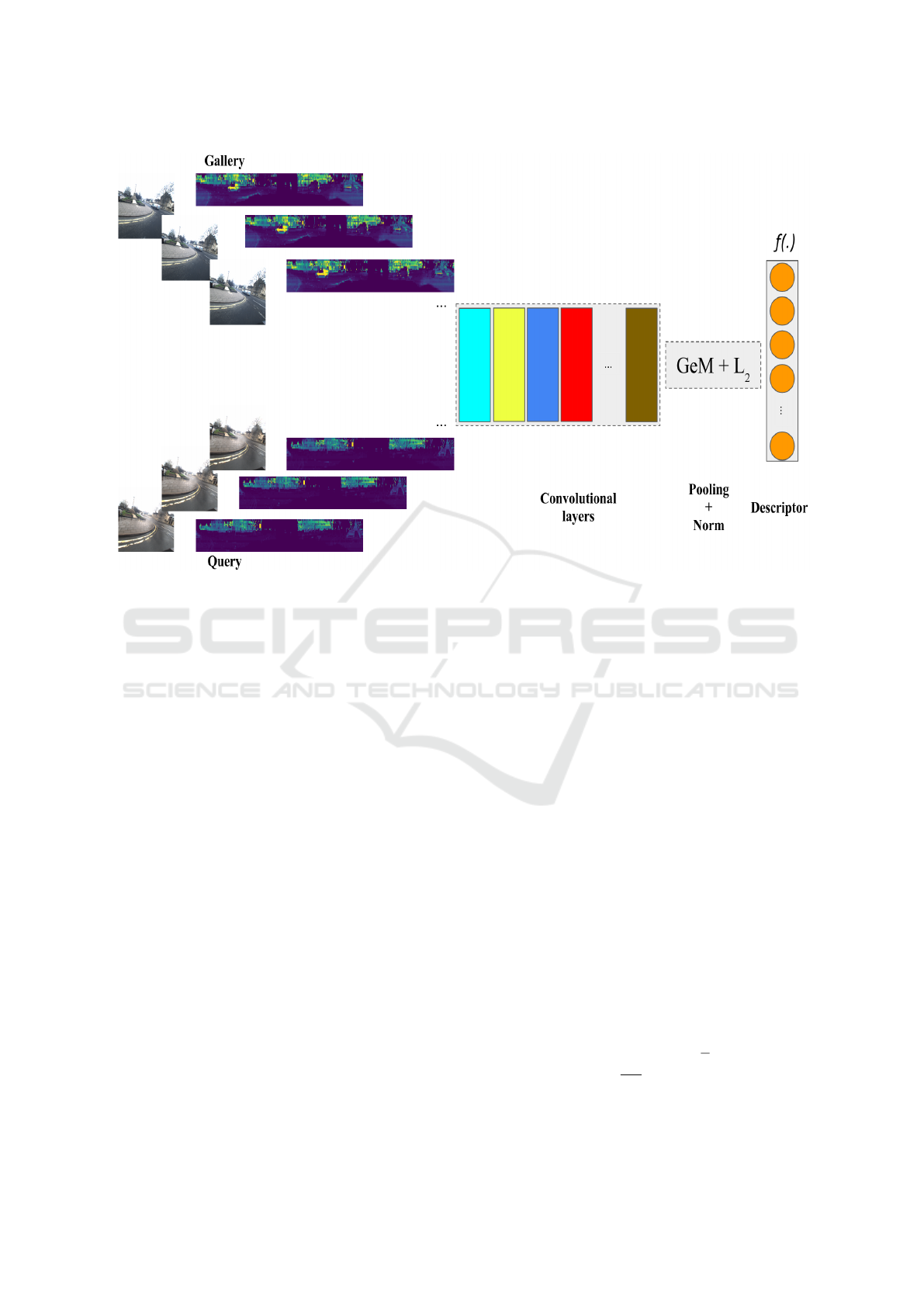
Figure 1: Overview of the network architecture with RGB image and LiDAR point clouds as sensor data modalities. Each
individual RGB image from the dataset is concatenated with its corresponding LiDAR point clouds which then input to the
DCNN to calculate the feature vector.
and the loss function enforces large distances between
negative pairs (images from two distant places) and
small distances between positive pairs (images from
the same place). Radenovic et al. (Radenovi
´
c et al.,
2019) use the contrastive loss (Hadsell et al., 2006)
that acts on matching (positive) and non-matching
(negative) pairs and is defined as follows:
L =
(
l(
~
f
a
,
~
f
b
) for matching images
max
0,M − l(
~
f
a
,
~
f
b
)
otherwise
(1)
where l is the pair-wise distance term (Euclidean
distance) and M is the enforced minimum margin be-
tween the negative pairs.
~
f
a
and
~
f
b
denote the deep
feature vectors of images I
a
and I
b
computed using
the convolutional head of a backbone network such
as AlexNet, VGGNet or ResNet. The typical feature
vector lengths K are 256, 512 or 2048, depending on
the backbone. Feature vectors are global descriptors
of the input images and pooled over the spatial di-
mensions. The feature responses are computed from
K convolutional layers X
k
following with max pool-
ing layers that select the maximum spatial feature re-
sponse from each layer (MAC vector)
~
f = [ f
1
f
2
... f
K
], f
k
= max
x∈X
k
x . (2)
Radenovic et al. originally used the MAC vec-
tors (Radenovi
´
c et al., 2016), but in their more recent
paper (Radenovi
´
c et al., 2019) compared MAC vec-
tors to average pooling (SPoC vector) and generalized
mean pooling (GeM vector) and found that GeM vec-
tors provide the best average retrieval accuracy.
The Radenovic et al. main pipeline is shared by
the most deep metric learning approaches for image
retrieval, but the unique components are the proposed
supervised whitening post-processing and effective
positive and negative sample mining. More details are
described in (Radenovi
´
c et al., 2016) and (Radenovi
´
c
et al., 2018) and available in the code provided by the
original authors.
Radenovic et al. (Radenovi
´
c et al., 2019) propose
GeM pooling layer to modify Maximum activation
of convolutions (MAC) (Azizpour et al., 2015; To-
lias et al., 2016a) and sum-pooled convolutional fea-
tures (SPoC) (Yandex and Lempitsky, 2015). This is
a pooling layer which takes χ as an input and pro-
duces a vector f = [ f
1
, f
2
, f
i
,..., f
K
]
T
as an output of
the pooling process which results in:
f
i
=
1
|χ
i
|
∑
x∈χ
i
x
p
i
!
1
p
i
(3)
MAC and SPoC pooling methods are special cases
VISAPP 2022 - 17th International Conference on Computer Vision Theory and Applications
652

of GeM depending on how pooling parameter p
k
is
derived in which p
i
→ ∞ and p
i
= 1 correspond to
max-pooling and average pooling, respectively. The
GeM feature vector is a single value per feature map
and its dimension varies depending on different net-
works, i.e. K = [256, 512, 2048]. It also adopts a
Siamese architecture to train the networks for image
matching.
4 EVALUATION PIPELINE
We evaluated our pipeline on a publicly available and
versatile outdoor dataset, e.g., Oxford Radar Robot-
Car (Barnes et al., 2020). We assigned three differ-
ent test sets, as query sequences, according to their
difficulty levels: (1) Test 01 with similar condition
to the gallery set (cloudy) but acquired at different
time; (2) Test 02 with moderately changed condi-
tions (sunny) and (3) Test 03 with different condition
from the gallery set (rainy). In the following, we de-
scribe the dataset and selection of training, gallery and
the three distinct query sequences along with training
process of our DCNN architecture.
4.1 Oxford Radar RobotCar Dataset
The Oxford Radar RobotCar dataset (Barnes et al.,
2020) is a radar extension to the Oxford RobotCar
dataset (Maddern et al., 2017). This dataset pro-
vides an optimized ground-truth using radar odome-
try data which is obtained from a Navtech CTS350-X
Millimetre-Wave FMCW. Data acquisition was per-
formed in January 2019 over 32 traversals in central
Oxford with a total route of 280 km urban driving.
This dataset addresses a variety of challenging con-
ditions including weather, traffic, and lighting alter-
ations. It also contains several sensor modalities to
perceive an environment and localize an agent accu-
rately (Figure 2).
The combination of one Point Grey Bumblebee
XB3 trinocular stereo and three Point Grey Grasshop-
per2 monocular cameras provide a 360° visual cov-
erage of scenes around the vehicle platform. Along
with the image sensor modality, this dataset also com-
prises a pair of high resolution real-time 3D Velodyne
HDL-32E LiDARs for 3D scene understanding. 6D
poses are acquired by NovAtel SPAN-CPT inertial
and GPS navigation system at 50 Hz and generated
by performing a large-scale optimization with ceres
solver incorporating visual odometry, visual loop clo-
sures, and GPS/INS constraints with the resulting tra-
jectories shown in Figure 2 (a).
The three monocular Grasshopper2 cameras with
fisheye lenses mounted on the rare side of the vehicle
are synchronized and logged 1024 × 1024 images at
an average frame rate of 11.1 Hz with 180° HFoV.
The Velodynes also provide 360° HFoV, 41.3°VFoV
with 100 m range and 2 cm range resolution for full
coverage around the vehicle.
In our evaluation pipeline, we are interested in
UNIX timestamp synchronized measured data of the
left-view camera images and left-side 3D LiDAR
point clouds, given their precise GPS/INS positions.
Therefore, in order to simplify our experiments, we
only obtain raw images from the left Point Grey
Grasshopper2 monocular camera along with raw 3D
point clouds from the left Velodyne LiDAR. The se-
lected sensor modalities points substantially towards
the left side of the road to encode the stable urban
environment characteristics, including buildings, cy-
clists, pedestrian traffic, traffic lights and passing-by
and/or parked cars.
4.2 Network Training
We fine-tune our DCNN architecture using the MAC,
SPoC and GeM pooling layers and weights of the
ResNet50 backbone which is initially pre-trained
on ImageNet (Russakovsky et al., 2015) dataset
for image-based, point cloud-based and image-point
cloud-based models. The idea of this procedure is to
use a pre-trained model, which to some extent is capa-
ble of recognizing locations, and adapt it to the place
recognition problem after fine-tuning.
We fine-tune our DCNN using contrastive loss
with hard matching (positive) and hard non-matching
(negative) pairs to improve the obtained image repre-
sentation, taking advantage of variability in the train-
ing data. The number of positive matches is the same
as the number of images in the pool of queries from
which they are selected randomly, whereas the num-
ber of negative matches is always fixed in the training.
Following (Radenovi
´
c et al., 2019), we learn
whitening through the same training data for two rea-
sons: (1) it mutually complement fine-tuning to boost
the performance, (2) applying whitening as a post-
processing step expedites training compared to learn-
ing it in an end-to-end manner (Radenovi
´
c et al.,
2016). We also utilize trainable GeM pooling layer
which significantly outperforms the retrieval perfor-
mance while preserving the dimension of the descrip-
tor. The comprehensive comparison results of MAC,
SPoC and GeM pooling layers are provided in Sec-
tion 5 for three test sets.
From the Oxford Radar RobotCar dataset, we
specify sequences for a training set for fine-tuning,
Evaluation of RGB and LiDAR Combination for Robust Place Recognition
653
(a)
(b)
(c)
(d)
(e)
(f)
(g)
(h)
(i)
(j)
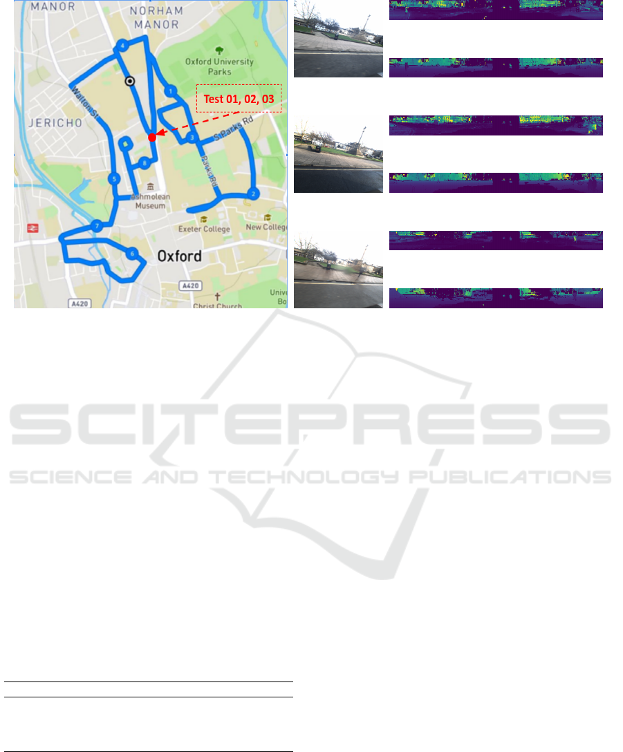
Figure 2: Three different sample tests, e.g., Test 01, Test 02 and Test 03 from Oxford Radard RobotCar outdoor dataset.
(a) Satellite-view with approximated GPS positions. (b), (e) and (h) Left-view of test images obtained from Grasshopper2:
cloudy, sunny, rainy, respectively. (c), (f) and (i) 3D LiDAR point clouds (intensity) obtained from Velodyne left. (d), (g) and
(j) 3D LiDAR point clouds (depth) obtained from Velodyne left.
a gallery set against which the query images from test
sequences are matched and three distinct test sets as
follows: (1) same day but different time, (2) differ-
ent day but approximately at the same time and (3)
different day and different time which also contains a
different weather condition. Table 1 summarizes dif-
ferent sets used for training, gallery and testing se-
quences. All experiments are conducted on a GPU
cluster with a single NVIDIA Quadro RTX 8000 GPU
with 32 GB memory using PyTorch 1.7 (Paszke et al.,
2019) deep learning framework.
Table 1: The Oxford Radar RobotCar sequences used in
our experiments. 1024 × 1024 Images obtained from Point
Grey Grasshopper2 monocular camera at 11.1 Hz mounted
on the rare and left side of the car. Point clouds obtained
from Velodyne HDL-32E 3D LIDAR at 20 Hz mounted on
the left side of the car.
Sequence Images Point Clouds Date Start [GMT] Condition
Train 37,724 44,414 Jan. 10 2019 11:46 Sunny
Gallery 36,660 43,143 Jan. 10 2019 12:32 Cloudy
Test 01 29,406 34,622 Jan. 10 2019 14:50 Cloudy
Test 02 32,625 38,411 Jan. 11 2019 12:26 Sunny
Test 03 28,633 33,714 Jan. 16 2019 14:15 Rainy
5 EXPERIMENTS
The conducted experiments in this paper address the
following research questions: (1) how precise the
fine-tuned DCNN architecture can recognize a scene,
given its primary contribution for the image retrieval
task? and whether or not its robustness changes over
challenging conditions, including the viewpoint and
the appearance variations, (2) which of the sensor
data modalities performs the best for the place recog-
nition problem in an outdoor environment? and (3)
how early fusion of RGB images and point clouds
(intensity and depth) could potentially boost the place
recognition performance?
Data Pre-processing. Given unrectified 8-bit raw
Bayer images, obtained from the left-side Point Grey
Grasshopper2 monocular camera, we first demosaic
images using RGGB Bayer pattern and then undistort
them using the look-up table for undistortion of im-
ages and mapping pixels in an undistorted image to
pixels in the distorted image. The resulting images are
shown in Figure 2 (b), (e) and (h). In our experiments,
we report the results of training with both raw Bayer
images and undistorted images to investigate the im-
pact of the RGB color space array, converted using
bilinear demosaicing algorithm (Losson et al., 2010).
The image dimensions are fixed at 1024 × 1024, sim-
ilar to original images. We also decode the raw Velo-
dyne samples into range, as depicted in Figure 2 (c),
(f) and (i), and intensity, as depicted in Figure 2 (d),
(g) and (j), which are then interpolated to consistent
azimuth angles between scans. Considering the early
fusion of RGB images and LiDAR point clouds, we
VISAPP 2022 - 17th International Conference on Computer Vision Theory and Applications
654

resize the intensity and range measurements such that
the aspect ratio is always fixed similar to the image
width, e.g., 1024, and height will be adjusted ac-
cordingly, thus the final dimensions of LiDAR point
clouds are 1024 × 46.
Performance Metric. After obtaining the image rep-
resentation of a given query image ( f (q)) using the
pipeline described in Section 4, calculating similar-
ity score indicates how well two images belong to the
same location in order to measure the performance.
In this way, the feature vector is matched to all image
representations of the gallery set f (G
i
),i = 1, 2,..., M
using Euclidean distance d
q,G
i
= || f (q)− f (G
i
)||
2
and
the smallest distance is selected as best match. The
best match position within the given distance thresh-
old (d
q,G
i
≤ τ) is identified as true positive and false
positive, otherwise.
Table 2: Recall@1 for Test 01 (different time but same day)
of the outdoor Oxford Radar RobotCar dataset.
Method τ = 25 m τ = 10 m τ = 5 m τ = 2 m
Only RGB (Bayer)
MAC (Tolias et al., 2016a) 71.07 69.24 64.55 60.63
SPoC (Yandex and Lempitsky, 2015) 73.42 70.02 65.85 61.77
GeM (Radenovi
´
c et al., 2019) 87.11 84.96 76.19 69.26
Only RGB (undistorted)
MAC (Tolias et al., 2016a) 76.55 69.56 66.42 62.14
SPoC (Yandex and Lempitsky, 2015) 79.23 71.41 67.00 64.99
GeM (Radenovi
´
c et al., 2019) 88.21 85.68 77.31 70.46
Only LiDAR (intensity)
MAC (Tolias et al., 2016a) 79.05 72.15 69.51 66.40
SPoC (Yandex and Lempitsky, 2015) 84.41 78.23 75.85 71.20
GeM (Radenovi
´
c et al., 2019) 95.57 94.22 86.72 77.34
Only LiDAR (depth)
MAC (Tolias et al., 2016a) 82.74 77.80 73.26 68.59
SPoC (Yandex and Lempitsky, 2015) 89.32 81.73 79.09 77.05
GeM (Radenovi
´
c et al., 2019) 97.71 96.82 88.13 80.06
RGB (undistorted) + LiDAR (intensity)
MAC (Tolias et al., 2016a) 79.11 71.38 68.71 64.02
SPoC (Yandex and Lempitsky, 2015) 83.52 77.12 74.71 71.05
GeM (Radenovi
´
c et al., 2019) 92.34 87.48 77.44 71.40
RGB (undistorted) + LiDAR (depth)
MAC (Tolias et al., 2016a) 78.75 71.98 69.02 64.88
SPoC (Yandex and Lempitsky, 2015) 83.01 76.25 75.38 71.00
GeM (Radenovi
´
c et al., 2019) 92.49 88.38 78.08 73.96
Following (Arandjelovic et al., 2018) and (Chen
et al., 2011), we measure the place recognition perfor-
mance by the fraction of correctly matched queries,
given the gallery dataset. We denote the fraction of
the top-N shortlisted correctly recognized candidates
as recall@N. Given the available ground-truth anno-
tations and τ for outdoor datasets, recall@N varies
accordingly. To evaluate the place recognition per-
formance using different sensor data modalities, we
report only the fraction of top-1 matches, (recall@1)
for multiple thresholds.
We provide the comparison results of fine-tuned
DCNN with three MAC, SpoC and GeM pooling lay-
ers in Table 2-4, for three test sets from the Oxford
Radar RobotCar dataset. GeM pooling layer consis-
tently outperforms MAC and SPoC with a clear mar-
gin given different sensor modalitiy inputs. Results of
Table 2, 3 and 4 also highlight a small outperformance
Table 3: Recall@1 for Test 02 (different day but same time)
of the outdoor Oxford Radar RobotCar dataset.
Method τ = 25 m τ = 10 m τ = 5 m τ = 2 m
Only RGB (Bayer)
MAC (Tolias et al., 2016a) 68.12 63.95 59.17 53.88
SPoC (Yandex and Lempitsky, 2015) 69.75 66.02 59.93 54.11
GeM (Radenovi
´
c et al., 2019) 71.75 68.41 61.30 56.08
Only RGB (undistorted)
MAC (Tolias et al., 2016a) 60.35 57.11 48.52 47.03
SPoC (Yandex and Lempitsky, 2015) 62.07 57.25 48.30 47.61
GeM (Radenovi
´
c et al., 2019) 65.06 58.94 51.40 49.82
Only LiDAR (intensity)
MAC (Tolias et al., 2016a) 84.32 81.25 78.25 69.01
SPoC (Yandex and Lempitsky, 2015) 85.93 83.02 80.01 70.02
GeM (Radenovi
´
c et al., 2019) 88.99 86.75 81.41 68.35
Only LiDAR (depth)
MAC (Tolias et al., 2016a) 96.15 94.21 92.71 85.41
SPoC (Yandex and Lempitsky, 2015) 95.95 94.09 93.41 86.16
GeM (Radenovi
´
c et al., 2019) 99.58 99.28 98.02 86.35
RGB (undistorted) + LiDAR (intensity)
MAC (Tolias et al., 2016a) 70.67 69.25 59.08 53.81
SPoC (Yandex and Lempitsky, 2015) 71.56 69.39 60.01 54.36
GeM (Radenovi
´
c et al., 2019) 77.51 70.58 60.17 55.71
RGB (undistorted) + LiDAR (depth)
MAC (Tolias et al., 2016a) 77.23 71.23 61.79 58.17
SPoC (Yandex and Lempitsky, 2015) 78.01 72.63 63.98 58.04
GeM (Radenovi
´
c et al., 2019) 81.20 74.19 64.89 60.21
when undistorted RGB images are used, compared to
Bayer images for all test sets. The reason is that the
DCNN mostly learns from the image center and four
dark corners of the raw Bayer images do not have a
significant effect on the fine-tuning stage. Test 02,
however, depicted a different results when converted
to undistorted images. One possible explanation is
the sunny condition of this test set in which major-
ity of the scenes are either blurred or occluded with
sunlight.
There is also a clear enhancement on the place
recognition performance results, given only LiDAR
point clouds as the primary sensory input for training
and fine-tuning the DCNN, compared to the RGB im-
ages. LiDAR point clouds remain largely invariant to
the lighting and seasonal changes which makes it a ro-
bust option in place recognition. The depth measure-
ments provides approximately 6 −10 % better perfor-
mance as the intensity data which are significant dif-
ferences in Test 02 and Test 03, corresponding to dif-
ferent conditions, compared to gallery set. In Test 01,
we obtain an average performance boost of 2.5 %.
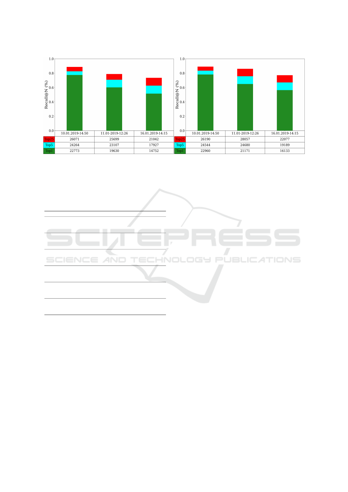
According to the extensive results of Figure 3, we
observe that fine-tuning of DCNN with GeM pooling
layers using early fusion of the RGB images and Li-
DAR point clouds outperform the case in which solely
RGB images are used. However, it fails to boost
the performance when compared to the case in which
only LiDAR point clouds is used as the primary sen-
sory input. A possible reason is the fusion approach
used in data pre-processing. In pre-processing, RGB
images (1024 × 1024) are still dominant part of the
learning process, compared to LiDAR point clouds
(1024 × 46).
Rank Analysis. We evaluated the early fusion per-
formance of RGB and LiDAR (depth) point clouds
Evaluation of RGB and LiDAR Combination for Robust Place Recognition
655
(a) (b)
Figure 3: Place recognition performance (Recalls and Tops) for given threshold (τ = 5.0 m), fine-tuned DCNN with GeM
pooling layer. (a) Early fusion of RGB images and LiDAR point clouds (intensity). (b) Early fusion of RGB images and
LiDAR point clouds (depth).
Table 4: Recall@1 for Test 03 (different day and different
time) of the outdoor Oxford Radar RobotCar dataset.
Method τ = 25 m τ = 10 m τ = 5 m τ = 2 m
Only RGB (Bayer)
MAC (Tolias et al., 2016a) 54.92 50.74 43.06 37.41
SPoC (Yandex and Lempitsky, 2015) 54.17 52.36 41.55 38.00
GeM (Radenovi
´
c et al., 2019) 56.84 52.25 43.76 38.14
Only RGB (undistorted)
MAC (Tolias et al., 2016a) 59.16 54.77 46.88 39.00
SPoC (Yandex and Lempitsky, 2015) 61.28 54.88 45.88 40.21
GeM (Radenovi
´
c et al., 2019) 62.16 56.25 46.58 40.26
Only LiDAR (intensity)
MAC (Tolias et al., 2016a) 64.92 58.03 49.77 44.01
SPoC (Yandex and Lempitsky, 2015) 65.41 59.11 51.55 45.14
GeM (Radenovi
´
c et al., 2019) 68.91 59.48 54.85 47.65
Only LiDAR (depth)
MAC (Tolias et al., 2016a) 72.24 68.89 57.47 47.56
SPoC (Yandex and Lempitsky, 2015) 73.88 69.06 56.69 49.63
GeM (Radenovi
´
c et al., 2019) 75.23 69.26 59.63 51.01
RGB (undistorted) + LiDAR (intensity)
MAC (Tolias et al., 2016a) 66.52 60.22 49.94 48.66
SPoC (Yandex and Lempitsky, 2015) 69.23 62.99 51.21 49.09
GeM (Radenovi
´
c et al., 2019) 70.36 63.77 51.52 49.56
RGB (undistorted) + LiDAR (depth)
MAC (Tolias et al., 2016a) 71.36 66.28 52.39 49.21
SPoC (Yandex and Lempitsky, 2015) 73.65 68.91 54.69 50.33
GeM (Radenovi
´
c et al., 2019) 76.46 69.21 56.34 51.21
with ranks and where exactly the failure occurs in the
Oxford Radar RobotCar dataset. The purpose is to
provide a visualization of the failure analysis on the
map, given three tests with different conditions, e.g.,
sunny, cloudy, rainy weather conditions.
Figure 4 illustrates our investigation of Rank5+
for Test 01, Test 02 and Test 03 with the number
of samples and their estimate positions on the map.
In our analysis, we refer to Rank5+ as a parameter
which identifies the most difficult test case has the
most number of hard failing samples, e.g., 9540 for
Test 01 compared to other tests. According to the re-
sults of Figure 4, we can generalize about the con-
ditions of the scene in which the more challenging
illumination leads to the higher ranks.
6 CONCLUSIONS
In this paper, we evaluated the place recognition per-
formance of DCNN using MAC, SpoC and GeM
pooling layers when fine-tuned with three different
sensor data modalities, including only RGB images,
only LiDAR point clouds (intensity and depth) and
early fusion of the RGB images with LiDAR point
clouds (intensity and depth). Our comprehensive
studies indicate that GeM pooling layers outperforms
MAC and SpoC pooling layers with margin. It also
demonstrates that LiDAR-based place recognition ap-
proach leads to more robust performance, given dif-
ferent appearance, and viewpoint variations, due to
longer range capability of the LiDAR compared to the
RGB-based approach.
Our experiments on three query tests with differ-
ent illumination conditions in the outdoor dataset il-
lustrated that using only LiDAR-based (depth) sen-
sor data outperforms the fine-tuning with LiDAR-
based (intensity) sensor data, especially in Test 03
with more challenging rainy conditions. Our eval-
uation has also shown that integrating early sensor-
fusion process with place recognition is challenging
and less robust compared to using only LiDAR point
cloud sensor data modality although it still obtains su-
perior results compared to only image-based sensor
data modality. This can be taken to the future studies
in which considering the idea of using one sensor data
to supervise the data of other sensors.
VISAPP 2022 - 17th International Conference on Computer Vision Theory and Applications
656
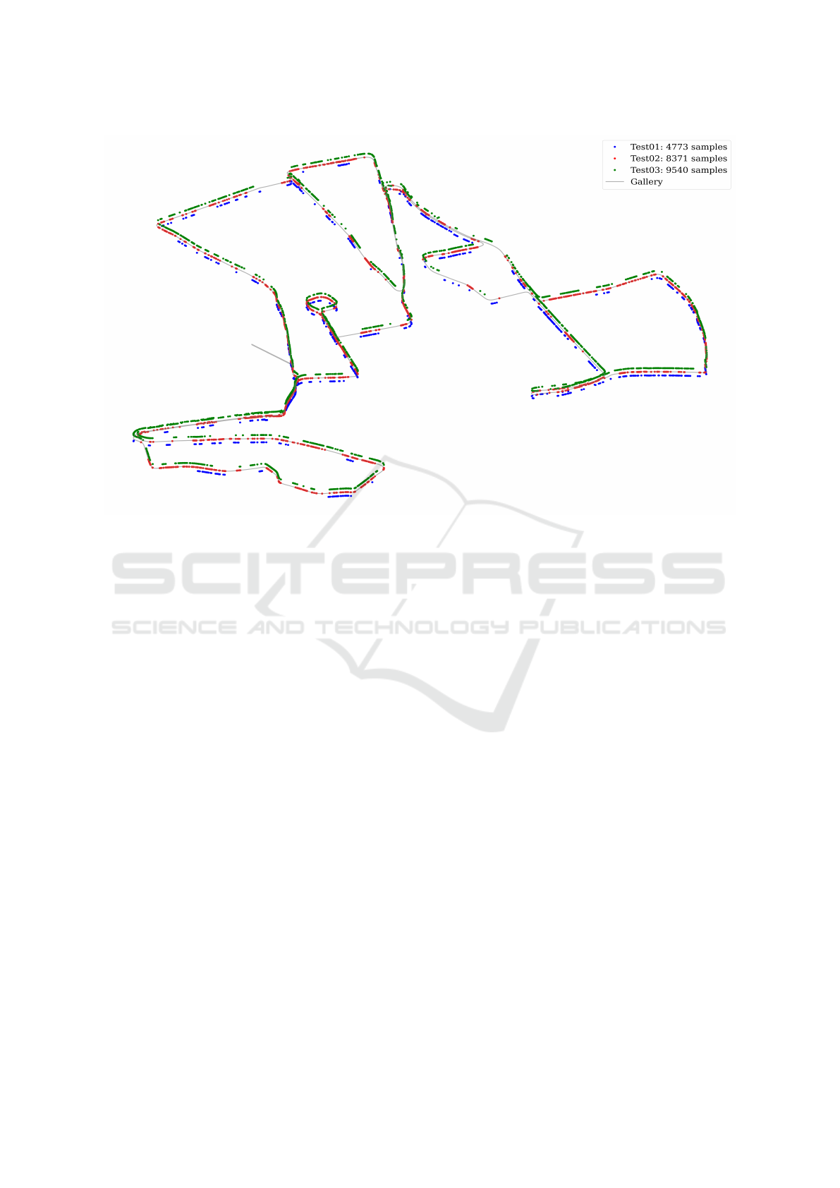
Figure 4: Rank Analysis for Test 01, Test 02 and Test 03 with different illuminations using early fusion of RGB and LiDAR
point clouds (depth) and τ = 5.0 m, fine-tuned DCNN with GeM pooling layer.
REFERENCES
Arandjelovic, R., Gronat, P., Torii, A., Pajdla, T., and Sivic,
J. (2018). NetVLAD: Cnn architecture for weakly su-
pervised place recognition. TPAMI.
Azizpour, H., Razavian, A. S., Sullivan, J., Maki, A., and
Carlsson, S. (2015). From generic to specific deep
representations for visual recognition. In 2015 IEEE
Conference on Computer Vision and Pattern Recogni-
tion Workshops (CVPRW), pages 36–45.
Barnes, D., Gadd, M., Murcutt, P., Newman, P., and Posner,
I. (2020). The oxford radar robotcar dataset: A radar
extension to the oxford robotcar dataset. In 2020 IEEE
International Conference on Robotics and Automation
(ICRA), pages 6433–6438.
Bay, H., Ess, A., Tuytelaars, T., and Van Gool, L. (2008).
Speeded-up robust features (surf). Computer Vision
and Image Understanding, 110(3):346–359. Similar-
ity Matching in Computer Vision and Multimedia.
Charles, R. Q., Su, H., Kaichun, M., and Guibas, L. J.
(2017). Pointnet: Deep learning on point sets for 3d
classification and segmentation. In 2017 IEEE Con-
ference on Computer Vision and Pattern Recognition
(CVPR), pages 77–85.
Chen, D. M., Baatz, G., K
¨
oser, K., Tsai, S. S., Vedantham,
R., Pylv
¨
an
¨
ainen, T., Roimela, K., Chen, X., Bach, J.,
Pollefeys, M., Girod, B., and Grzeszczuk, R. (2011).
City-scale landmark identification on mobile devices.
In CVPR 2011, pages 737–744.
Cummins, M. and Newman, P. (2008). Fab-map: Proba-
bilistic localization and mapping in the space of ap-
pearance. The International Journal of Robotics Re-
search, 27(6):647–665.
Dewan, A., Caselitz, T., and Burgard, W. (2018). Learning
a local feature descriptor for 3d lidar scans. In Proc. of
the IEEE/RSJ International Conference on Intelligent
Robots and Systems (IROS), Madrid, Spain.
Dub
´
e, R., Dugas, D., Stumm, E., Nieto, J., Siegwart, R.,
and Cadena, C. (2017). Segmatch: Segment based
place recognition in 3d point clouds. In 2017 IEEE
International Conference on Robotics and Automation
(ICRA), pages 5266–5272.
Filliat, D. (2007). A visual bag of words method for interac-
tive qualitative localization and mapping. In Proceed-
ings 2007 IEEE International Conference on Robotics
and Automation, pages 3921–3926.
Hadsell, R., Chopra, S., and LeCun, Y. (2006). Dimen-
sionality reduction by learning an invariant mapping.
In 2006 IEEE Computer Society Conference on Com-
puter Vision and Pattern Recognition (CVPR’06), vol-
ume 2, pages 1735–1742.
He, L., Wang, X., and Zhang, H. (2016). M2dp: A novel
3d point cloud descriptor and its application in loop
closure detection. In 2016 IEEE/RSJ International
Conference on Intelligent Robots and Systems (IROS),
pages 231–237.
J
´
egou, H., Douze, M., Schmid, C., and P
´
erez, P. (2010).
Aggregating local descriptors into a compact image
representation. In 2010 IEEE Computer Society Con-
ference on Computer Vision and Pattern Recognition,
pages 3304–3311.
J
´
egou, H., Douze, M., Schmid, C., and P
´
erez, P. (2010).
Evaluation of RGB and LiDAR Combination for Robust Place Recognition
657

Aggregating local descriptors into a compact image
representation. In 2010 IEEE Computer Society Con-
ference on Computer Vision and Pattern Recognition,
pages 3304–3311.
Kalantidis, Y., Mellina, C., and Osindero, S. (2016). Cross-
Dimensional Weighting for Aggregated Deep Convo-
lutional Features. In Computer Vision – ECCV 2016
Workshops, pages 685–701. Springer, Cham, Switzer-
land.
Klokov, R. and Lempitsky, V. (2017). Escape from cells:
Deep kd-networks for the recognition of 3d point
cloud models. In 2017 IEEE International Conference
on Computer Vision (ICCV), pages 863–872.
Liu, Z., Zhou, S., Suo, C., Yin, P., Chen, W., Wang, H., Li,
H., and Liu, Y. (2019). Lpd-net: 3d point cloud learn-
ing for large-scale place recognition and environment
analysis. In 2019 IEEE/CVF International Conference
on Computer Vision (ICCV), pages 2831–2840.
Losson, O., Macaire, L., and Yang, Y. (2010). Comparison
of color demosaicing methods. In Advances in Imag-
ing and Electron Physics, volume 162, pages 173–
265. Elsevier.
Lowe, D. G. (2004). Distinctive Image Features from Scale-
Invariant Keypoints. Int. J. Comput. Vision, 60(2):91–
110.
Lowry, S., S
¨
underhauf, N., Newman, P., Leonard, J. J.,
Cox, D., Corke, P., and Milford, M. J. (2016). Vi-
sual place recognition: A survey. IEEE Transactions
on Robotics, 32(1):1–19.
Maddern, W., Pascoe, G., Linegar, C., and Newman, P.
(2017). 1 year, 1000 km: The oxford robotcar
dataset. The International Journal of Robotics Re-
search, 36(1):3–15.
Martinez, J., Doubov, S., Fan, J., B
ˆ
arsan, l. A., Wang, S.,
M
´
attyus, G., and Urtasun, R. (2020). Pit30m: A
benchmark for global localization in the age of self-
driving cars. In 2020 IEEE/RSJ International Confer-
ence on Intelligent Robots and Systems (IROS), pages
4477–4484.
Masone, C. and Caputo, B. (2021). A survey on deep visual
place recognition. IEEE Access, 9:19516–19547.
Milford, M. J. and Wyeth, G. F. (2012). Seqslam: Vi-
sual route-based navigation for sunny summer days
and stormy winter nights. In 2012 IEEE International
Conference on Robotics and Automation, pages 1643–
1649.
Paszke, A., Gross, S., Massa, F., Lerer, A., Bradbury, J.,
Chanan, G., Killeen, T., Lin, Z., Gimelshein, N.,
Antiga, L., Desmaison, A., K
¨
opf, A., Yang, E., De-
Vito, Z., Raison, M., Tejani, A., Chilamkurthy, S.,
Steiner, B., Fang, L., Bai, J., and Chintala, S. (2019).
Pytorch: An imperative style, high-performance deep
learning library. ArXiv, abs/1912.01703.
Qi, C. R., Yi, L., Su, H., and Guibas, L. J. (2017). Point-
net++: Deep hierarchical feature learning on point sets
in a metric space. arXiv preprint arXiv:1706.02413.
Radenovi
´
c, F., Tolias, G., and Chum, O. (2019). Fine-tuning
cnn image retrieval with no human annotation. IEEE
Transactions on Pattern Analysis and Machine Intel-
ligence, 41(7):1655–1668.
Radenovi
´
c, F., Tolias, G., and Chum, O. (2016). CNN
image retrieval learns from BoW: Unsupervised fine-
tuning with hard examples. In ECCV.
Radenovi
´
c, F., Tolias, G., and Chum, O. (2018). Deep shape
matching. In ECCV.
Russakovsky, O., Deng, J., Su, H., Krause, J., Satheesh,
S., Ma, S., Huang, Z., Karpathy, A., Khosla, A.,
Bernstein, M., Berg, A. C., and Fei-Fei, L. (2015).
ImageNet Large Scale Visual Recognition Challenge.
International Journal of Computer Vision (IJCV),
115(3):211–252.
Rusu, R. B., Blodow, N., and Beetz, M. (2009). Fast point
feature histograms (fpfh) for 3d registration. In 2009
IEEE International Conference on Robotics and Au-
tomation, pages 3212–3217.
Shi, B., Bai, S., Zhou, Z., and Bai, X. (2015). Deeppano:
Deep panoramic representation for 3-d shape recogni-
tion. IEEE Signal Processing Letters, 22(12):2339–
2343.
Su, H., Maji, S., Kalogerakis, E., and Learned-Miller, E.
(2015). Multi-view convolutional neural networks for
3d shape recognition. In 2015 IEEE International
Conference on Computer Vision (ICCV), pages 945–
953.
Tolias, G., Sicre, R., and J
´
egou, H. (2016a). Particular
Object Retrieval With Integral Max-Pooling of CNN
Activations. In ICL 2016 - RInternational Confer-
ence on Learning Representations, International Con-
ference on Learning Representations, pages 1–12, San
Juan, Puerto Rico.
Tolias, G., Sicre, R., and J
´
egou, H. (2016b). Particular ob-
ject retrieval with integral max-pooling of cnn activa-
tions.
Torii, A., Arandjelovi
´
c, R., Sivic, J., Okutomi, M., and Pa-
jdla, T. (2015). 24/7 place recognition by view syn-
thesis. In 2015 IEEE Conference on Computer Vision
and Pattern Recognition (CVPR), pages 1808–1817.
Uy, M. A. and Lee, G. H. (2018). Pointnetvlad: Deep point
cloud based retrieval for large-scale place recognition.
In 2018 IEEE/CVF Conference on Computer Vision
and Pattern Recognition, pages 4470–4479.
Yandex, A. B. and Lempitsky, V. (2015). Aggregating local
deep features for image retrieval. In 2015 IEEE In-
ternational Conference on Computer Vision (ICCV),
pages 1269–1277.
Zhang, W. and Xiao, C. (2019). Pcan: 3d attention map
learning using contextual information for point cloud
based retrieval. In 2019 IEEE/CVF Conference on
Computer Vision and Pattern Recognition (CVPR),
pages 12428–12437.
Zhang, X., Wang, L., and Su, Y. (2021). Visual place recog-
nition: A survey from deep learning perspective. Pat-
tern Recognition, 113:107760.
Zou, C., He, B., Zhu, M., Zhang, L., and Zhang, J. (2019).
Learning motion field of lidar point cloud with con-
volutional networks. Pattern Recognition Letters,
125:514–520.
VISAPP 2022 - 17th International Conference on Computer Vision Theory and Applications
658
