Disruption Management of ASAE’s Inspection Routes

Miguel Milheiro Ferreira

1,2

, Henrique Lopes Cardoso

1,2

, Lu

ıs Paulo Reis

1,2

, Telmo Barros

1,2

and Jo

ao Pedro Machado

Laborat

orio de Intelig

encia Artiﬁcial e Ci

encia de Computadores (LIACC), Portugal

Faculdade de Engenharia da Universidade do Porto, Rua Dr. Roberto Frias, s/n, 4200-465 Porto, Portugal

Autoridade de Seguranc¸a Alimentar e Econ

omica (ASAE), Rua Rodrigo da Fonseca, 73, 1269-274 Lisboa, Portugal

Keywords:

Vehicle Routing, Disruption Management, Real-time Scheduling, Routes Rescheduling, Hill-climbing,

Simulated Annealing, Tabu-search, Large Neighbourhood Search.

Abstract:

The emergence of technologies capable of producing real-time data opened new horizons to planning and op-

timising vehicle routes. Dynamic vehicle routing problems (DVRPs) use real-time information to dynamically

calculate the most optimised set of routes. The typical approach is to initially calculate the vehicle routes and

dynamically revise them in real-time. This work uses the case study of ASAE, a Portuguese administrative

authority specialising in food safety and economic surveillance. The dynamic properties of ASAE’s opera-

tional environment are studied, and a solution is proposed to review and efﬁciently modify the precalculated

plan. We propose a weighted utility function based on three aspects: the summed utility of the inspections,

the similarity between solutions, and the arrival time. A Disruption Generator generates disruptions on the

inspection routes: travel and inspection times, vehicle and inspection breakdowns, utility changes, and unex-

pected or emerging inspections. We compare the performance of four meta-heuristics: Hill-Climbing (HC),

Simulated Annealing (SA), Tabu-Search (TS) and Large neighbourhood Search (LNS). The HC algorithm has

the fastest convergence, while SA takes longer to solve the test instances. LNS was the method with higher

solution quality, while HC provided solutions with lower utility.

1 INTRODUCTION

During the last decades, urban transportation experi-

enced a rapid and signiﬁcant evolution supported by

the emergence and development of several vital tech-

nologies. On the other hand, computational power has

approximately doubled every two years since 1975

(Moore’s Law). Computational power also beneﬁts

from new computation paradigms such as parallel

computing, since speciﬁc portions of the code are exe-

cuted in Graphics Processing Units (GPU), massively

boosting performance. These technologies and pro-

cesses bring the opportunity to improve vehicle per-

formance, mainly by optimising vehicle routes. Sev-

eral beneﬁts can be accounted for: improved safety,

less trafﬁc congestion, monetary savings, and reduced

environmental impact (Genders and Razavi, 2016).

The typical approach to address multi-vehicle route

planning relies on centralised control, having an in-

frastructure that gathers and combines vehicle data,

leading to more efﬁcient and intelligent route optimi-

sations. Further optimisations can be achieved con-

cerning dynamic environment factors by using algo-

rithms that beneﬁt from the information collected in

real-time. The evolution of communication medi-

ums eases knowledge transference between the vehi-

cle ﬂeet and the centralised control. This work arises

from a project (Barros et al., 2020; Barros et al., 2021)

that seeks to improve the Portuguese Economic and

Food Safety Authority (ASAE) inspection activities.

ASAE’s activities are vital as they ensure competition

fairness among economic operators and improve food

safety.

The contributions of this work regard the dynamic

and real-time optimisation of inspection routes to

surveil economic operators. Any real-world vehicle

routing scenario is susceptible to disruptions – uncer-

tain events that inﬂuence an operational plan – mak-

ing a planned route unfeasible or sub-optimal. A stan-

dard paradigm to maintain feasibility and optimality

is to revise inspection routes in real-time and mod-

ify them once a disruption occurs. Such a complex

task requires the use of systems capable of collecting

the geographic position of ﬂeet vehicles in real-time

810

Ferreira, M., Cardoso, H., Reis, L., Barros, T. and Machado, J.

Disruption Management of ASAE’s Inspection Routes.

DOI: 10.5220/0010914000003116

In Proceedings of the 14th International Conference on Agents and Artiﬁcial Intelligence (ICAART 2022) - Volume 3, pages 810-817

ISBN: 978-989-758-547-0; ISSN: 2184-433X

and knowledge about the location of every economic

operator. Each economic operator to be inspected

has an associated utility, reﬂecting the value an in-

spection brings. The problem explored in this work

was modelled as a Dynamic Vehicle Routing Problem

with Time Windows (DVRPTW). Solving this opti-

misation problem corresponds to ﬁnding the inspec-

tion routes that bring the most utility for the system

while respecting all constraints. Such task is often

computationally intractable, and approximation tech-

niques become vital in ﬁnding a good solution in rea-

sonable time.

2 RELATED WORK

Research in the ﬁeld of vehicle routing has increased

massively, with enterprises aiming to lower their costs

and increase their proﬁts. This area has attracted

many researchers, mainly on the subject of dynamic

routing, especially in the last three decades (Psaraftis

et al., 2016). On his survey, Pillac et al. catalogued

154 references on the topic (Pillac et al., 2013).

VRPs consist of determining the set of routes to

be traversed by a vehicle ﬂeet to serve a group of cus-

tomers or visit a set of locations (Eglese and Zam-

birinis, 2018). They were ﬁrst introduced by Dantzig

and Ramser (Dantzig and Ramser, 1959). Since then,

multiple instances of the problem and algorithms to

ﬁnd solutions have been described in the literature.

The most straightforward and famous vehicle routing

problem is the Traveling Salesman Problem (TSP):

Having a set of cities to visit, calculate the shortest

path, starting from an initial city, that visits each city

exactly once and then returns to the starting city (Hah-

sler and Hornik, 2007). The set of routes outputted

when solving the VRP might be impossible to execute

as some unforeseen events happen. Also, there might

be a window to optimise the pre-calculated operations

plan further.

Dynamic Vehicle Routing Problems (DVRP) are

the dynamic family of problems deriving from VRP,

where the routes can suffer the inﬂuence of dynamic

elements. The routes have to be revised and modiﬁed

in real-time. There is a panoply of factors that play

an essential role in this trend, such as hardware evo-

lution, the appearance of devices and systems that can

gather and transmit vehicle data in real-time, the ac-

cess to information APIs and the Global Positioning

System (GPS). All these data and systems can be used

and combined in real-time to gather and create useful

information that will play a crucial role in optimising

vehicle routes (Pillac et al., 2013). They enhance and

explain the decisions taken in Dynamic Routing.

Wilson and Colvin ﬁrst described a DVRP formu-

lation (Wilson and Colvin, 1977). They studied the

dial-a-ride problem (DARP), where client requests

appear dynamically during execution time. They used

an insertion heuristic approach to obtain an approxi-

mate solution with low computational effort (Psaraftis

et al., 2016).

DVRPs are divided into two clusters: the Dynamic

and deterministic VRP and the Dynamic and stochas-

tic VRP. Although both variants can be considered

as dynamic, they differ in the presence of stochastic

information about dynamic events. In dynamic and

stochastic VRPs, this information is available before-

hand and may be useful to plan future decisions.

As the initially calculated plan will be modiﬁed

and revised, the costs entailed by deviations should

also be taken into account. Therefore, disruption

management is often a multi-objective problem, as

the costs of modifying the plan should be added to

the costs already present on the original plan (Eglese

and Zambirinis, 2018).

3 INSPECTION ROUTES

PROBLEM

3.1 Problem Description

ASAE is currently responsible for inspecting more

than 1.5 million economic operators in the Portuguese

territory. ASAE’s structure is segmented into three re-

gional units, each being divided into operational units,

in a total of twelve units. Operational units are de-

pots where the brigades start and ﬁnish their sched-

uled tasks. Each operational unit has a different num-

ber of available vehicles and personnel and is respon-

sible for inspecting a subset of the economic opera-

tors in the system. Each inspection is performed by

a brigade that is always capable of inspecting any

economic operator. All the economic operators are

geo-referenced and have an associated inspection util-

ity, calculated using information such as its history of

customer complaints, which are reported to ASAE.

The dynamic factors in the real-world environ-

ment that might inﬂuence the routes are manyfold. In

this work, six disruptive elements are considered: (i)

dynamic inspection times; (ii) dynamic travel times

between two sites; (iii) vehicle breakdowns; (iv) in-

spection breakdowns; (v) utility changes; and (vi) un-

expected or emerging inspections.

Disruption Management of ASAE’s Inspection Routes

811

3.2 Problem Formulation

The problem can be formulated as a Multi-depot Dy-

namic Vehicle Routing Problem with Time Windows

(MDDVRPTW). This formulation describes the vast

majority of vehicle routing problems. They usually

comprise several depots from where the vehicles are

routed. Time windows are essential, as economic op-

erators’ working schedules must be considered in case

of inspection. The approach described in this work

considers only a single operational unit and all the

economic operators under its jurisdiction.

The problem addressed in this paper is a max-

imisation problem, aiming to ﬁnd the best feasible

solution according to a complex utility function (ad-

dressed in Section 3.5). We model the problem with a

ﬁnite number of constraints perceived from the real-

world scenario. The following are the most relevant

ones:

• Inspection brigades have a deﬁned time to leave

the initial depot (operational unit) and arrive at the

same place when the workday ends, at a speciﬁed

timestamp.

• An economic operator may be inspected at most

once per operational plan, and the inspection must

start during the economic operator business hours.

• Each inspection brigade can only inspect one eco-

nomic operator at a time.

• A vehicle or brigade that has suffered a break-

down is no longer available for inspection tasks

in that workday.

• Emerging inspections are mandatory and have to

be completed prior to the workday end.

Continuous optimisation is done during the day

upon a disruption. This approach was ﬁrst used in

(Gendreau et al., 1999) with an adaptation of the par-

allel Tabu-Search algorithm to solve a Dynamic VRP

with time windows, motivated by courier services.

The current problem solution is maintained in mem-

ory, being updated continuously once the available

problem information changes.

3.3 Disruption Generator

We propose and implement a system that tackles dis-

ruptions in real-time. For the purpose of this work,

“real-time” has to be simulated to allow testing the

proposed approach. A Disruption Generator artiﬁ-

cially generates realistic disruptions that should be ad-

dressed by the algorithms. It receives an operational

plan corresponding to the set of inspection routes for

one working day and returns a new operational plan

with disruptions in the inspection routes. Six ma-

jor disruptions are considered: disruption of the in-

spection times and travel times, vehicle breakdowns,

inspection breakdowns, changes in inspection utility

and emerging inspections.

ASAE inspects economic operators from several

business sectors that can be classiﬁed into ten main

clusters. Although one can reasonably predict the in-

spection time necessary to inspect an economic oper-

ator from a speciﬁc sector, many factors can inﬂuence

these times. Travel time disruptions can be caused by

a panoply of external elements, from trafﬁc conditions

or changes in the vehicle’s speed. They are usually

associated with delays. A Gaussian distribution was

used to sample new inspection and travel times, sim-

ulating a disruption. The two parameters to calculate

the Gaussian curve are the predicted inspection/travel

time, and a customizable deviation factor to adjust the

disruption severity.

Vehicle breakdown disruptions are common in

most VRPs and concern ﬂeet vehicles in operation.

Any vehicle in operation can suffer a breakdown

caused by various reasons that prevents it from pro-

ceeding in its current inspection route. ASAE opera-

tions do not involve customer demands that have to be

satisﬁed. A system can simply re-optimise the whole

operational plan.

Inspection breakdowns are very particular to

ASAE’s operations scenario and regard unforeseen

events during inspections. Inspection breakdowns

happen when a brigade is forced to stop inspecting

an economic operator and cannot proceed with its in-

spection route.

Disruptions regarding changes in inspection util-

ity concern the utility values of the economic opera-

tors. These values can change due to micro and macro

factors. The implementation of this disruption was

based on ASAE’s ten clusters of economic activities:

the disruption implies that all economic operators per-

taining to a speciﬁc economic activity will see an in-

crease in their inspection utility.

An emerging inspection is one that has top priority

and must be performed. To simulate one such inspec-

tion, the disruption generator randomly selects one

economic operator absent in the initial operational

plan and adds it in a random place in an inspection

route. However, emerging inspections are manda-

tory and have to be completed prior to the workday

end. They can be performed by any brigade, and any

brigade is able to perform multiple inspections of this

type.

ICAART 2022 - 14th International Conference on Agents and Artiﬁcial Intelligence

812

3.4 Solution Generation

The implemented algorithms imply using methods to

generate new solutions based on solutions provided as

input. For this work, six different operators were im-

plemented. These operators share the common task

of taking a solution as input and outputting a new so-

lution after changing one or more inspection routes.

The economic operators are seen as the blocks that

will be moved and altered to originate a new solution.

Each operator involves stochastic decisions to gener-

ate distinct solutions.

All operators comprise exchange, add, and re-

move operations and act both on the same or differ-

ent inspection routes. These operations can be ap-

plied to a single economic operator (Figure 1) and

over a sequence of two consecutive economic oper-

ators, dubbed 2*OPT operations (Figure 2).

Figure 1: Single Economic Operator operations.

Figure 2: 2*OPT operations.

3.5 Utility Function

The ﬂexible utility function used in this work contem-

plates three different domains with deﬁned weights.

The utility of a particular solution is obtained by

weighing (1) the total sum of all economic operators’

utilities, (2) the similarity between the initial solution

and the solution obtained after solving the disruption,

and (3) the average time each brigade arrives at the

depot at the work day’s end.

A key element in a dynamic vehicle routing prob-

lem is the magnitude of the changes in the routes

once disruption occurs compared to the routes ini-

tially calculated. These changes entail added costs

that may sometimes outcome the savings achieved by

re-optimising the routes once disruptions occur. The

similarity between any two corresponding routes in-

creases as they encompass the same number of eco-

nomic operators, and the economic operators visited

by the corresponding routes in the initial and posterior

solution are equal and inspected in the same order.

Each economic operator registered in the system

has an individual utility value that determines how de-

sirable it is to be inspected and its value to ASAE’s

inspection system. This value ranges from 0 to 1 and

is calculated based on a weighted sum of n functions

that take into consideration the following attributes

(Barros et al., 2021): (i) the economic operator’s ac-

tivity sector. (ii) the number and severity of pending

complaints; and (iii) its history of inspections.

The last parameter in the utility function is the

time each brigade arrives at the depot at the end of

the day. Solutions totaling more utility gathered from

inspections are not necessarily better, as they might

entail that brigades arrive too close to the maximum

allowed time, leaving less margin for disruptions.

3.6 Unfeasible Solutions

This work explores unfeasible solutions as they might

accelerate discovering new solutions on some algo-

rithms and contribute to faster convergence. Since the

problem is modelled as a DVRP, disruptions can often

make inspection routes unfeasible, so it is vital to have

an approach that weighs these solutions. Unfeasible

solutions do not fulﬁl one or more of the problem’s

restrictions (see Section 3.2).

In order for the algorithm to distinguish and weigh

each solution, unfeasible ones have to be penalised

in the utility function. This work uses a continuous

non-stationary penalty function (Liu and Lin, 2007).

The complex penalty function in Eq. 1 is divided into

two functions: a dynamic function f (x) (Eq. 2) and a

continuous assignment function H(x) (Eq. 3) that can

address both linear and non-linear constraints.

F(x) = f (x) −C(k)H(x) (1)

Eq. 1 was adapted to a maximisation problem.

This equation returns the new utility value after ap-

plying the respective penalty values to unfeasible so-

lutions. Function f (x) is the utility value of a spe-

ciﬁc solution calculated using the utility function pre-

viously proposed.

C(k) = (c × k)

(2)

The dynamic function in Eq. 2 depends on the iter-

ation number k and increases as the search progresses.

Disruption Management of ASAE’s Inspection Routes

813

c and α are two problem-dependent constants manu-

ally tuned to the values of 0.05 and 1, respectively.

H(x) =

∑

i=1

[θ(q

(x)) × q

(x)

ρ(q

(x))

] (3)

Function H(x) (Eq.3) represents the penalty fac-

tor. This function will be the sum of all the penalty

types applied to a particular solution. Function q

(x)

is a numeric value representing how far a solution is

from the feasible space for one penalty type. Function

ρ(q

(x)) adjusts the violating function and is set either

for the value one when a solution is near the feasible

space or two otherwise.

θ(q

(x)) = a × (1 −

(x)

) + b (4)

Function θ(q

(x)) (Eq. 4) is a continuous assign-

ment function also adapted from Liu and Lin (Liu

and Lin, 2007). In this work, a and b are problem-

dependent constants adjusted to the values of 150 and

1, respectively.

3.7 Algorithms

This work implements and compares the performance

of four distinct meta-heuristic optimisation algo-

rithms: Hill-Climbing, Simulated Annealing, Tabu-

Search, and Large Neighbourhood Search.

3.7.1 Hill-Climbing

The Hill-Climbing (HC) algorithm has the most

straightforward implementation. The algorithm starts

with a preliminary solution that can be feasible or

unfeasible, representing the several inspection routes

composing an operational plan. The algorithm fol-

lows the same logic in each iteration, ﬁrst generat-

ing a new candidate solution based on the current one

(using one of the operators described previously), and

then evaluating its utility using the proposed utility

function. A candidate solution is accepted if it has

better utility than the best solution found during the

previous search iterations.

3.7.2 Simulated Annealing

The Simulated Annealing (SA) algorithm is an al-

gorithm that allows the acceptance of worse solu-

tions to avoid getting trapped in local maximum.

The algorithm’s initial temperature is chosen using

a method adapted from Atiqullah (Atiqullah, 2004).

This method creates a normal distribution of ten thou-

sand neighbours and calculates the standard deviation

to be later used in Eq. 5.

∆C =

∑

attempts

i=1

|∆C

i, j

attempts

(5)

The cooling schedule used in this implementation

is an adaptation of the parametric cooling schedule

used by Atiqullah (Atiqullah, 2004). The ﬁnal tem-

perature was set to 0.0001, and the values for the

constants a and b were assigned to a = 2 and b =

1/3. Two new temperature rules were implemented to

complement the proposed cooling schedule and based

on the two phases of a SA search, global position-

ing, and solution reﬁnement. In the global positioning

phase, the temperature remains at its max for 5% of

the total number of iterations allowed. To better ad-

dress the solution reﬁnement phase, the temperature is

set to a null value, only accepting the best solutions.

The stopping criteria used for the algorithm results

from the combination of a deﬁned number of itera-

tions and a deﬁned number of Markov chains without

improvement.

= t

× α

−[

]

(6)

b =

(7)

P = log

log(

)

log(a)

(8)

Q = log





(9)

This work implements a reheating method that

restarts the search process a deﬁned amount of times,

with the initial solution and temperature. If the solu-

tion from one reheat was better, the best global solu-

tion is updated.

3.7.3 Tabu-search

The Tabu-search (TS) implementation results from

a combination of methods analysed in the litera-

ture. This work implements a diversiﬁcation strat-

egy where solutions are generated by prioritising less

frequent solution elements and intensiﬁcation phases

where the search might restart from an elitist solution

(Cordeau and Laporte, 2005).

The proposed implementation comprises three

different memory structures: two short-term (tabu-

lists) to store tabu operations for the next N-iterations

(exchange and addition/removal operations) and one

long-term to store the frequency of solution elements.

The solution generation method generates and

evaluates the utility of a subset of the neighbourhood

with 100 elements obtained randomly from the cur-

rent solution using a set of operators. Six operators

are used with an equal frequency for this purpose.

ICAART 2022 - 14th International Conference on Agents and Artiﬁcial Intelligence

814

Two Aspiration criteria were implemented. A tabu

solution is accepted if its utility is higher than the best

solution’s utility. The second Aspiration criterion ver-

iﬁes if the utility of a new solution generated by a tabu

move is higher than the utility of the solution gener-

ated by the same move in a past iteration.

3.7.4 Large Neighbourhood Search

Large Neighborhood Search (LNS) was implemented

jointly with Tabu-search. This algorithm minimises a

large neighbourhood of solutions into a small neigh-

bourhood (Shaw, 1998; Azi et al., 2014). In this prob-

lem’s context, the building blocks of a solution are the

inspection routes since they are independent.

In each iteration, the algorithm ﬁxes a number

of inspection routes, meaning they will not take part

in the optimisation process in that iteration. Only

two inspection routes will be optimised in each al-

gorithm’s iteration, facilitating the search for prob-

lems with many brigades. A TS solves the artiﬁcial

sub-problem instance, returning a solution that is ap-

pended with the remaining routes rebuilding the orig-

inal solution. This LNS implementation always starts

with a feasible solution. A TS instance is used when

the initial solution is unfeasible.

4 RESULTS

This work performs all the executions in the same

problem instance, adapted from a real-world scenario.

The problem instance analysed is a sub-problem of

the real-world environment with fewer inspection

routes and economic operators. A single depot is

used. The static parameters used in the tests are:

• Operational unit: Unidade Operacional III - Mi-

randela, district of Braganc¸a.

• All economic operators belong to the this opera-

tional unit, totaling 532 different operators.

• Brigades start working at 8 am and ﬁnish at 6 pm.

• As initial solution, four inspection routes are con-

sidered, generated by Barros’s approach (Barros

et al., 2021) using several metaheuristic methods.

• The inspection time is 1 hour.

Each test result corresponds to the average met-

rics of three system runs with the same conditions.

The tests were executed using an Intel i7 8700, with

16 GB RAM, running Windows 10. Several metrics

are studied: the average utility of economic opera-

tors inspected, the utility of economic operators in the

best solution found, the average value of the utility

function, the utility function value of the best solution

found, the average similarity ratios, the average and

minimum time to get the best solution, the average

iteration counter to get the best solution, the average

number of economic operators in the best solution.

4.1 Algorithm Comparison

The ﬁrst experiment has the main objective of making

a raw comparison between the four algorithms. The

utility function used in this test is the economic opera-

tor’s utility gathered by the inspections. The only dis-

ruptions generated for these tests are travel time and

inspection time disruptions. The algorithms are exe-

cuted for thirty seconds, two and ﬁve minutes, while

the number of brigades (and thus number of inspec-

tion routes) is two, three and four. All the tests results

are shown in Table 1. A string identiﬁes each test. The

ﬁrst sub-string identiﬁes the number of brigades, the

second represents the algorithm used, and the last rep-

resents the execution time. The tests using the LNS

with two inspection routes are discarded since the re-

sults were expected to be the same as with TS.

Regarding run times, SA performs worse since it

spends a signiﬁcant time in the exploratory phase. HC

ﬁnds the best solution in the shortest execution time,

scoring the best execution time in ﬁve out of nine

tests. TS comes next, scoring the best execution time

in four out of nine tests. HC performs the worse in

terms of solution quality, having the lowest average

solution utility in eight out of the nine tests. However,

it can still ﬁnd reasonable solutions since its execu-

tion depends on stochasticity. For problem instances

with two inspection routes, the TS algorithm ﬁnds the

highest utility solutions and the highest average solu-

tion utility. For larger problem instances with more

inspection routes, LNS revealed to be the best algo-

rithm to ﬁnd the best solutions consistently.

4.2 Disruption Types Comparison

This test section studies how the different algorithms

respond to the various disruptions types. The util-

ity function comprised 2 components with a weight

of 0.66 for the utility sum of all the inspected eco-

nomic operators and 0.33 for solution similarity (see

Section 3.5). Algorithm execution time is topped at

4 minutes. The initial operational plan is composed

of four inspection routes. All the tests and results are

shown in Table 2 and Table 3.

SA provides solutions with a poor similarity ratio.

Other algorithms balance utility gathering with keep-

ing the solution relatively similar to the initial opera-

tional plan, obtaining solutions that are roundly 30%

Disruption Management of ASAE’s Inspection Routes

815

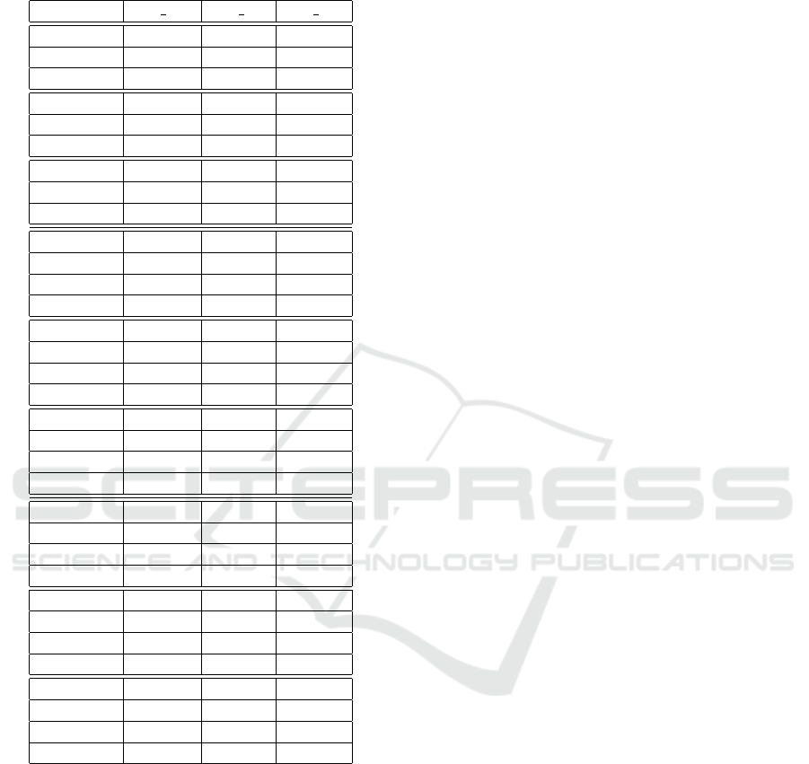
Table 1: Algorithm comparison. UA: sum of economic op-

erator utilities; ST: search execution time; OP: number of

economic operators.

ID avg UA avg ST avg OP

2-HC-30 7.87 11.45 17.67

2-SA-30 8.25 21.83 17.33

2-TS-30 8.24 13.33 17.00

2-HC-2 7.28 17.16 18.00

2-SA-2 8.22 66.87 16.33

2-TS-2 8.30 10.50 18.00

2-HC-4 7.26 37.49 18.33

2-SA-4 8.29 194.38 17.00

2-TS-4 8.30 25.60 17.67

3-HC-30 9.90 22.74 27.67

3-SA-30 10.69 29.15 25.00

3-TS-30 10.53 19.23 27.00

3-LNS-30 10.53 32.84 26.00

3-HC-2 10.52 34.78 27.00

3-SA-2 10.75 100.43 25.00

3-TS-2 10.79 35.49 26.33

3-LNS-2 10.72 104.57 26.00

3-HC-4 10.19 31.39 28.00

3-SA-4 10.74 147.56 25.00

3-TS-4 10.77 141.06 25.67

3-LNS-4 11.50 153.64 28.33

4-HC-30 12.46 19.85 37.33

4-SA-30 12.91 33.95 35

4-TS-30 12.71 20.58 35.33

4-LNS-30 12.80 32.44 35

4-HC-2 12.83 78.32 36.33

4-SA-2 12.93 109.19 33.66

4-TS-2 12.81 33.50 36.00

4-LNS-2 12.95 95.07 34.33

4-HC-4 12.53 78.81 36.00

4-SA-4 13.17 148.90 35.33

4-TS-4 12.97 202.92 35.33

4-LNS-4 13.92 116.60 34.33

similar to the original one. All tests with emerging in-

spections have a substantially higher utility since they

have higher utilities.

HC quickly ﬁnds the best solution, while SA per-

forms worse on this metric. TS and LNS have simi-

lar average time intervals. HC fails to solve two out

of the three problem instances involving emerging in-

spections, outputting unfeasible solutions. The algo-

rithm seems to get stuck in the initial solution, having

difﬁculty progressing in the search. An algorithm like

HC is unsuitable for solving such disruption since it

does not allow worse solutions, not allowing emerg-

ing inspections to be readjusted freely in the plan.

Tests involving inspection and vehicle break-

downs have a lower utility since less brigades are

working. The solutions obtained in solving a problem

instance with changes in utility usually include more

economic operators of the affected activity sector.

The current implementation of LNS inﬂuences the

algorithm’s performance to solve emerging inspec-

tions. Economic operators corresponding to emerg-

ing inspections cannot be exchanged between routes

as easily compared to other implementations, as only

2 routes are optimised in each iteration.

5 CONCLUSIONS

This work proposes a valid approach to tackle disrup-

tions in a DVRP scenario. It culminated in imple-

menting a system capable of generating and address-

ing disruptions to a set of inspection routes. Overall,

the algorithms provided reasonable solutions in most

of the tests. HC has the fastest convergence and fails

to address the emerging inspections. SA fails to de-

liver solutions with higher similarity ratios. TS of-

fered an outstanding balance between ﬁnding the best

solution and in the shortest amount of time. TS also

solved all problem instances and returned solutions

similar to the initial ones when the utility function

beneﬁts such behaviour. LNS consistently offered a

better solution quality when compared to other algo-

rithms. Nevertheless, this algorithm is sub-optimal

compared to SA and TS when solving the emerging

inspections disruption.

A further enhancement of the process can be ob-

tained by dividing the optimisation process into two

stages: to quickly get a reasonable solution and then

optimizing it to produce a better solution(Ritzinger

et al., 2016). Stochastic information can be used to

further adapt the initial solution to dynamic elements

that are likely to happen during the execution of the

planned routes. Methods such as sampling (Pillac

et al., 2013) could be used.

ACKNOWLEDGEMENTS

This work is supported by project IA.SAE, funded

by Fundac¸

ao para a Ci

encia e a Tecnologia (FCT)

through program INCoDe.2030. This research is

supported by LIACC (FCT/UID/CEC/0027/2020).

Telmo Barros is supported by a PhD scholarship from

FCT (2021.05064.BD).

ICAART 2022 - 14th International Conference on Agents and Artiﬁcial Intelligence

816

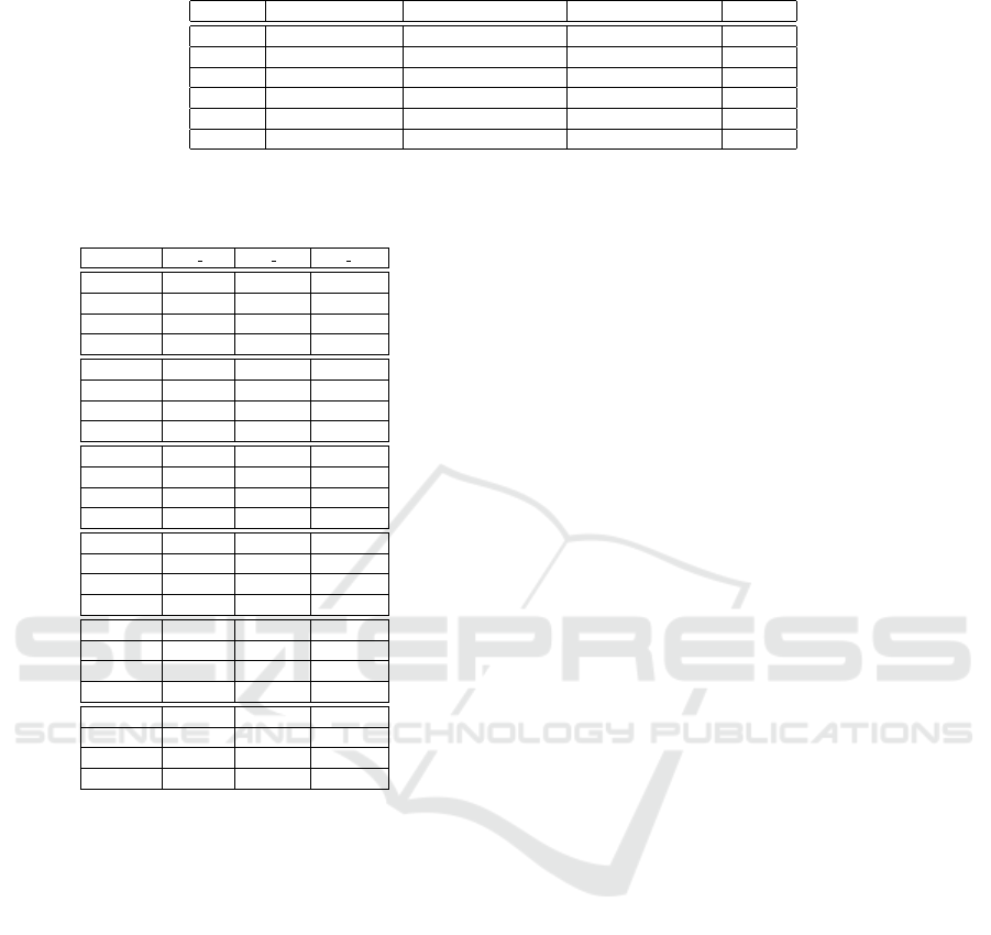
Table 2: Tests identiﬁcation and parameters - Experiment 2; Alg stands for the corresponding algorithm initials.

ID Algorithms Disruption Type Dis Param Value

Alg-IT HC, SA, TS, LNS Inspection Time Disruption Strength 5

Alg-TT HC, SA, TS, LNS Travel Time Disruption Strength 5

Alg-VB HC, SA, TS, LNS Vehicle Breakdown No. Vehicles 1

Alg-UC HC, SA, TS, LNS Utility Changes Econ. Operator class III,V,VI

Alg-IB HC, SA, TS, LNS Inspection Breakdown No. Inspections 1

Alg-EI HC, SA, TS, LNS Emerging inspections No. Inspections 2

Table 3: Disruption management results. UF: utility func-

tion, UA: sum of economic operator utilities, Sim: solution

similarity.

ID avg UF avg UA avg Sim

HC-IT 13.09 11.55 0.22

SA-IT 12.88 12.88 0.00

TS-IT 13.51 11.15 0.34

LNS-IT 14.27 12.62 0.24

HC-TT 12.93 11.48 0.21

SA-TT 12.98 12.98 0.00

TS-TT 12.99 10.66 0.33

LNS-TT 13.04 10.80 0.31

HC-VB 10.74 9.67 0.20

SA-VB 10.76 10.76 0.00

TS-VB 10.72 9.30 0.270

LNS-VB 10.64 9.96 0.21

HC-UC 10.47 9.88 0.11

SA-UC 10.90 10.90 0.00

TS-UC 10.80 9.69 0.21

LNS-UC 10.70 9.47 0.23

HC-IB 13.57 11.75 0.26

SA-IB 12.89 12.89 0.00

TS-IB 13.77 11.58 0.31

LNS-IB 13.56 11.10 0.35

HC-EI -44.00 204.67 0.69

SA-EI 212.94 212.43 0.07

TS-EI 212.98 210.60 0.34

LNS-EI 211.99 209.37 0.37

REFERENCES

Atiqullah, M. M. (2004). An efﬁcient simple cooling sched-

ule for simulated annealing. Lecture Notes in Com-

puter Science (including subseries Lecture Notes in

Artiﬁcial Intelligence and Lecture Notes in Bioinfor-

matics), 3045:396–404.

Azi, N., Gendreau, M., and Potvin, J.-Y. (2014). An adap-

tive large neighborhood search for a vehicle routing

problem with multiple routes. Computers I& Opera-

tions Research, 41:167–173.

Barros, T., Oliveira, A., Cardoso, H. L., Reis, L. P.,

Caldeira, C., and Machado, J. P. (2021). Economic

and food safety: Optimized inspection routes genera-

tion. In Rocha, A. P., Steels, L., and van den Herik, J.,

editors, Agents and Artiﬁcial Intelligence, pages 482–

503, Cham. Springer International Publishing.

Barros, T., Santos, T., Oliveira, A., Cardoso, H. L., Reis,

L. P., Caldeira, C., and Machado, J. P. (2020). In-

teractive inspection routes application for economic

and food safety. In Rocha,

A., Adeli, H., Reis, L. P.,

Costanzo, S., Orovic, I., and Moreira, F., editors,

Trends and Innovations in Information Systems and

Technologies, pages 640–649, Cham. Springer Inter-

national Publishing.

Cordeau, J.-F. and Laporte, G. (2005). Tabu search heuris-

tics for the vehicle routing problem. In Sharda, R.,

Voß, S., Rego, C., and Alidaee, B., editors, Meta-

heuristic Optimization via Memory and Evolution:

Tabu Search and Scatter Search, pages 145–163.

Springer US, Boston, MA.

Dantzig, G. B. and Ramser, J. H. (1959). The Truck Dis-

patching Problem. Management Science, 6(1):80–91.

Eglese, R. and Zambirinis, S. (2018). Disruption manage-

ment in vehicle routing and scheduling for road freight

transport: a review. Top, 26(1):1–17.

Genders, W. and Razavi, S. N. (2016). Impact of Connected

Vehicle on Work Zone Network Safety through Dy-

namic Route Guidance. Journal of Computing in Civil

Engineering, 30(2):04015020.

Gendreau, M., Guertin, F., Potvin, J.-Y., and Taillard, E.

(1999). Parallel tabu search for real-time vehicle rout-

ing and dispatching. Transportation Science, 33:381–

390.

Hahsler, M. and Hornik, K. (2007). TSP - Infrastructure for

the traveling salesperson problem. Journal of Statisti-

cal Software, 23(2):1–21.

Liu, J. L. and Lin, J. H. (2007). Evolutionary computa-

tion of unconstrained and constrained problems using

a novel momentum-type particle swarm optimization.

Engineering Optimization, 39(3):287–305.

Pillac, V., Gendreau, M., Gu

eret, C., and Medaglia, A. L.

(2013). A review of dynamic vehicle routing prob-

lems. European Journal of Operational Research,

225(1):1–11.

Psaraftis, H. N., Wen, M., and Kontovas, C. A. (2016). Dy-

namic vehicle routing problems: Three decades and

counting. Networks, 67(1):3–31.

Ritzinger, U., Puchinger, J., and Hartl, R. F. (2016). A sur-

vey on dynamic and stochastic vehicle routing prob-

lems. International Journal of Production Research,

54(1):215–231.

Shaw, P. (1998). Using constraint programming and local

search methods to solve vehicle routing problems. In

Maher, M. and Puget, J.-F., editors, Principles and

Practice of Constraint Programming — CP98, pages

417–431. Springer Berlin Heidelberg.

Wilson, N. and Colvin, N. (1977). Computer Control of the

Rochester Dial-A-Ride System. CTS report. MIT.

Disruption Management of ASAE’s Inspection Routes

817

REFERENCES

Atiqullah, M. M. (2004). An efficient simple cooling sched-