Generative Model for Autoencoders Learning by Image Sampling

Representations

V. E. Antsiperov

Kotelnikov Institute of Radioengineering and Electronics of RAS, Mokhovaya 11-7, Moscow, Russian Federation

Keywords: Ideal Image, Counting Statistics, Autoencoders, Generative Model, Machine Learning, Feature Extraction.

Abstract: The article substantiates a generative model for autoencoders, learning by the input image representation

based on a sample of random counts. This representation is used instead of the ideal image model, which

usually involves too cumbersome descriptions of the source data. So, the reduction of the ideal image concept

to sampling representations of fixed (controlled) size is one of the main goals of the article. It is shown that

the corresponding statistical description of the sampling representation can be factorized into the product of

the distributions of individual counts, which fits well into the naive Bayesian approach and some other

machine learning procedures. Guided by that association the analogue of the well-known EM algorithm – the

iterative partition–maximization procedure for generative autoencoders is synthesized. So, the second main

goal of the article is to substantiate the partition–maximization procedure basing on the relation between

autoencoder image restoration criteria and statistical maximum likelihood parameters estimation. We succeed

this by modelling the input count probability distribution by the parameterized mixtures, considering the

hidden mixture variables as autoencoder’s internal (coding) data.

1 INTRODUCTION

Machine learning methods have been attracting the

attention of researchers for more than half a century.

The first methods and approaches were largely

borrowed / adapted from the statistical theory, whose

foundations were established about a hundred years

ago, primarily by the works of R. Fisher. Discoveries

in related fields in the middle of the XX-th century,

primarily in neuropsychology, greatly influenced the

development and originality of machine learning. We

note in this connection the McCulloch and Pitts

model of the neuron (1943) and the Hebb’s rule for

the perceptron (1949). This was followed by a

relatively long period of experience accumulation and

analysis of the possibilities of implementing network

learning methods on computers. A breakthrough in

this direction was the invention in the mid-1980s by

Rumelhart, Hinton, and Williams of the error

backpropagation algorithm for training neural

networks (1986).

Over the past 30-40 years, the evolution of neural

networks has come a long way. Along with the

supervised approaches, unsupervised ones began to

https://orcid.org/0000-0002-6770-1317

develop, deep learning is gaining more importance.

Under the influence of these trends, several new

classes of neural networks have appeared and

developed. Note here DBNs (Deep Belief Networks),

CNNs (convolutional neural networks), RNNs

(recurrent neural networks), as well as LSTMs (Long

Short-Term Memory) and AEs (autoencoders).

Without exaggeration, autoencoders are at the

forefront of unsupervised learning. This is partly due

to the symmetry of their architecture, which is a

coupled codec pair. In non-AE approaches, where

either an encoder or a decoder is absent, expensive

optimization algorithms should be used to find the

code or sampling techniques to achieve restoration. In

contrast to them, AE contains both elements in its

structure, moreover, encoder and decoder actively

influence the solution of each other's problems.

In this work, we propose a new approach to

learning AE by the images presented in a special way

– by special sampling representations. The first half

of the paper discusses in detail the relation of

sampling representation with the ideal image model.

The second part of the paper is devoted to learning

AE in generative model using the sampling

354

Antsiperov, V.

Generative Model for Autoencoders Learning by Image Sampling Representations.

DOI: 10.5220/0010915200003122

In Proceedings of the 11th International Conference on Pattern Recognition Applications and Methods (ICPRAM 2022), pages 354-361

ISBN: 978-989-758-549-4; ISSN: 2184-4313

representations at the input. The questions of

generative model formalization, encoding/decoding

procedures optimization and their connection to the

method of maximum likelihood estimation in

statistical theory are considered in detail.

2 IMAGE SAMPLING

REPRESENTATION

In several previous papers (Antsiperov, 2021 a, b) we

proposed the representation of images by the samples

of random counts (basing on counting statistics (Fox,

2006)). This approach was partially substantiated in

(Seitz, 2011) by the physical mechanisms of the real

image formation and detection.

Today’s relevance of the proposed representation

is due, on the one hand, to progress in the SPAD

(single photon avalanche diodes) video matrixes, that

photocounts (Fossum, 2020), (Morimoto, 2020). On

the other hand, it is due to the ever-increasing trends

in the adaptation of human visual perception

mechanisms for digital image processing (Beghdadi

2013), (Rodieck, 1998).

Both of the tendences mentioned incorporate

several common features. The SPAD-matrixes, as

well as human retina include some sensitive 2D-

surface, which consists of a very large number of

detectors/receptors. These detectors are so small, that

each of them can detect the individual photon of the

incident radiation. The detailed, comprehensive

review of these trends in modern photon-counting

sensors can be found in the book (Fossum, 2017). The

use of visual perception mechanisms for digital image

processing is widely discussed in (Gabriel, 2015). So,

the listed features can be taken as the basis of the

concept of the ideal imaging device, generalizing

besides the photon-counting sensors mentioned also

the photographic plates with gelatin-silver emulsion,

etc.

Formally, the definition of an ideal imaging

device is as follows. It is a two-dimensional surface

𝛺 with coordinates 𝑥⃗𝑥



,𝑥



, on which identical

point detectors are allocated close to each other. Point

detectors, or in terms of (Fossum, 2020) "jots", have

by a definition a vanishingly small area 𝑑𝑎 of light-

sensitive surfaces. Accordingly, if the total number of

detectors is 𝑁, then the total area of surface 𝛺 is equal

to 𝐴𝑁𝑑𝑎. Under the assumption that 𝐴 is fixed

and 𝑑𝑎 → 0 , the number 𝑁 is assumed to be

arbitrarily large: 𝑁→∞.

When the ideal imaging device registers the

stationary radiation with intensity 𝐼



𝑥⃗



,𝑥⃗∈𝛺, some

of point detectors generate the counts – random

events that in the case of SPAD matrixes are the

releases of an electron from p-n junction of the

photodiode, in the case of retina  activations of

rhodopsin molecules in photoreceptors and in the case

of photographic plates  appearing of metallic silver

atom clusters in or on a silver halide crystal. Within

the framework of the semiclassical theory of

interaction between radiation and matter, the counts

are associated with incident photons captured by

atoms / molecules of the detector's material. At the

limit 𝑑𝑎 → 0 the probability of a count (in any

interpretation) for a given point detector is the

product 𝛼𝑇𝐼𝑥⃗𝑑𝑎, where 𝛼𝜂ℎ𝜈̅



, ℎ𝜈̅  the

average energy of the incident photon (ℎ  Planck's

constant, 𝜈̅  characteristic frequency of radiation),

the dimensionless coefficient 𝜂1 is the quantum

efficiency of the detector’s material (Fox, 2006), 𝑇 is

exposure time. Thus, when the incident radiation of

intensity 𝐼



𝑥⃗



is registered, the state of each point

detector 𝑥⃗∈𝛺 can be described by a binary random

variable 𝜎



⃗

∈0,1, taking the values 𝜎



⃗

1 and

𝜎



⃗

0, depending on whether has the detector

generate a count. The conditional (at a given intensity

𝐼𝑥⃗) probabilities of 𝜎



⃗

have the form of Bernoulli

distribution:

𝑃



𝜎



⃗

1|𝐼𝑥

⃗



𝛼𝑇𝐼𝑥

⃗

𝑑𝑎,

𝑃



𝜎



⃗

0|𝐼𝑥

⃗



1𝛼𝑇𝐼𝑥

⃗

𝑑𝑎.

(1)

Note that, according to (1), formally, the mean

number of counts for given point detector 𝑥⃗ is equal

to 𝜎



⃗

𝛼𝑇𝐼𝑥⃗𝑑𝑎 (it is assumed, that 𝜎



⃗

1).

Accordingly, the integral 𝑛

∑

𝜎



⃗



⃗

∈



𝛼𝑇

∬

𝐼



𝑥⃗



𝑑𝑎



defines the mean number of all

registered over time 𝑇 counts.

Based on the concept of an ideal imaging device

and considering the main features of its registration

mechanism (1), it is possible to formulate a model of

an ideal image as a resultant set of counts, generated

during the registration process. Namely, under the

ideal image we mean the (ordered) set 𝑋



𝑥⃗



,…,𝑥⃗





, 𝑥⃗



∈𝛺 of 𝑛 random counts registered

(𝜎



⃗



1) by the ideal imaging device during the time

𝑇. Thus, an ideal image is a kind of random object, a

random set of count coordinates 𝑥⃗



∈𝛺, which

should be distinguished from any of its realization.

We use the name "ideal image" for the proposed

construction, following the authors of (Pal, 1991), in

which they introduced this term for the first time in

the early 90s. It is worth noting that the randomness

of the ideal image is related not only to the random

Generative Model for Autoencoders Learning by Image Sampling Representations

355

nature of count coordinates 𝑥⃗



, but also it is

determined by the random value of 𝑛 – the number of

counts in the set.

A complete statistical description of ideal image

𝑋 in the form of finite-dimensional probability

distribution densities 𝜌𝑥⃗



,…,𝑥⃗



,𝑛|𝐼



𝑥⃗



, 𝑥⃗



∈

𝛺,𝑛  0,1,... can be obtained by assuming

conditional independence of all counts 𝑥⃗



(under the

condition of the given 𝐼



𝑥⃗



and 𝑛). It is well known

(Poisson’s theorem, (Gallager, 2013)), that under

such assumptions, asymptotically, with 𝑁→∞ the

probability distribution of Bernoulli process (trial)



𝜎



⃗



,𝑥⃗∈𝛺 (1) converges to the Poisson process

distributions (Streit, 2010) on 𝛺:

𝜌𝑥

⃗



,…,𝑥

⃗



,𝑛|𝐼



𝑥

⃗





∏

𝜌𝑥

⃗



|𝐼



𝑥

⃗









𝑃





𝑊



(2)

where

𝑃





𝑊









!

exp



𝛼𝑇𝑊



𝜌𝑥

⃗



|𝐼



𝑥

⃗











⃗







,𝑊

∬

𝐼



𝑥

⃗



𝑑𝑎



where 𝑃





𝑊



is the Poisson probability distribution

(Gallager, 2013), (Streit, 2010) of 𝑛 – number of

counts in ideal image 𝑋, 𝑛𝛼𝑇𝑊 is its mean, 𝑊 is

the overall registered radiation power. Conditional

𝜌𝑥⃗|𝐼



𝑥⃗



 is the density of single count probability

distribution. In connection with (2), it is interesting to

note that the (statistical) intensity of 2D point Poisson

process 𝜎



⃗

𝑑𝑎

⁄

coincides with the physical intensity

𝐼



𝑥⃗



of the recorded radiation up to the constant 𝛼𝑇.

From the theoretical point of view the concept of

an ideal image is a very attractive statistical object

due to the simplicity of its statistical description (2)

and its interpretation as an inhomogeneous point

Poisson process that had been well studied for a long

time. However, in practical tasks it is not always

possible to use this concept directly in the form in

which it is formulated. Namely, for common recorded

radiation intensities 𝐼



𝑥⃗



, the direct use of the ideal

image realization 𝑋



𝑥⃗



,…,𝑥⃗





would require

enormous computational resources when the number

of counts 𝑛 is big enough. So, considering that on a

clear day the flux of photons from the sun falling on

a surface with 𝐴 ~ 1 𝑚𝑚



per second is of order

~ 10



 10



photons (Rodieck, 1998), the devices

in a photon counting mode will generate the

information flow of the value of 𝑛 ~ 10



(1 Pbit/sec).

Obviously, it is very problematic to process such

information with the modern computing technique.

To avoid the "curse of dimension" of ideal image

representation, we propose the following solution

(Antsiperov, 2021 a). Let us represent the image not

by the complete sets of ideal image counts 𝑋



𝑥⃗



,…,𝑥⃗





, but only by some subset 𝑋





𝑥⃗





,…,𝑥⃗





, 𝑗



∈1,…,𝑛 of acceptable fixed size

𝑘, where 𝑥⃗





are randomly selected counts from 𝑋.

Formally, considering 𝑋 as a general population of

counts, we propose to use only a random sample 𝑋



of them to represent the image. Obviously, in full

agreement with the classical statistical paradigm,

such a "sample" representation will still represent the

ideal image 𝑋 . Let us name such a sample 𝑋



"representation by a sample of random counts" or, in

short, the sampling representation.

The statistical description of sampling

representation follows easily from (2) by integrating

density 𝜌𝑥⃗



,…,𝑥⃗



,𝑛|𝐼



𝑥⃗



 over the not selected in

𝑋



count coordinates and summing the result over the

number 𝑙 of not selected counts. In the actual case

1≪𝑘≪𝑛 the statistical description of sampling

representation 𝑋



is given with high accuracy by the

probability distribution density of the form:

𝜌𝑋



|𝐼



𝑥

⃗





∏

𝜌



𝑥

⃗



|𝐼



𝑥

⃗









𝜌



𝑥

⃗



|𝐼



𝑥

⃗













⃗







,𝑊

∬

𝐼



𝑥

⃗



𝑑𝑎



(3)

Regarding description (3), it should be noted that

it has very simple structure, depending only on the

shape (normalized version) of the registered intensity

𝐼



𝑥⃗



𝑊

⁄

. This immediately leads to some attractive

representation properties. First, it reveals the

conditional independence of all 𝑘 counts 𝑥⃗



and their

identical conditional distribution (iid property).

Second, the density of the individual count

𝜌𝑥⃗



|𝐼𝑥⃗ is very simply related to intensity 𝐼𝑥⃗ of

radiation – they are proportional to each other. Third,

the description satisfies the following universality

property: it does not depend either on the quantum

efficiency of the detector material 𝜂 , or on the

incident radiation average frequency 𝜈̅ , or on frame

time 𝑇 . These sampling presentation properties

provide a convenient, suitable input data for many

well–developed statistical and machine learning

approaches, including the naive Bayesian approach

(Barber, 2012).

A consequence of the universality property is also

the fact that statistical description of the sampling

representation (3) does not depend on physical units

of intensity 𝐼𝑥⃗. So, if, for example, the intensity

𝐼𝑥⃗ is given by pixels of some bitmap image,

obtained by digitization with a quantization

parameter 𝑄Δ𝐼, then description (4) will not

directly dependent on 𝑄, but it will depend only on

ICPRAM 2022 - 11th International Conference on Pattern Recognition Applications and Methods

356

the pixel color depth 𝜐. This remark allows to

generate sampling representations not only for the

source data of the photon counting sensors, but also

for common digital images obtained by traditional

camera. To do this, one should use the all-image

pixels 𝑛



 to form an approximation

𝑛



∑

𝑛



𝐼



𝑥⃗





𝑊

⁄⁄

of the original normalized

intensity and then simulate the process of sampling

independent counts from it according (3). Regarding

the computational organization of sampling,

fortunately, in the field of machine learning, there is

a large arsenal of methods, collectively called Monte

Carlo methods (Murphy, 2012), that can do this very

efficiently.

It should be noted that for some methods even

pixels 𝑛



 normalization is not required at all – it is

sufficient that all pixels are bounded from above by

the constant 2



, where 𝜐 is the color depth of the

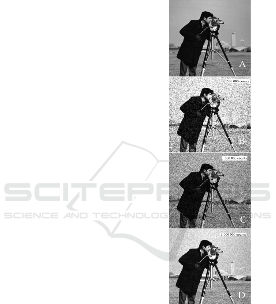
image. For example, Figure 1 shows count

representations of the picture “cameraman”

(distributed by the MathWorks, Inc. with permission

from the MIT), presented in subfigure A. The

sampling representations with sizes 500 000,

1 000 000 and 5 000 000, 1 000 000 and 5 000 000

counts – B, C and D were carried out by one of the

simplest sampling procedures – acceptance-rejection

method using a uniform proposal distribution.

3 LEARNING AE BY SAMPLING

REPRESENTATIONS

Usually, autoencoders (AE) are considered as a

special class of artificial neural networks (ANNs)

(Hinton, 1994), but for our purposes it is desirable to

define them from a more general point of view.

Namely, we will consider AEs as a special class of

information systems, understood as an "integrated set

of components for collecting, storing and processing

data" (Information system. In Encyclopedia

Britannica, 2020). In current context, the processing

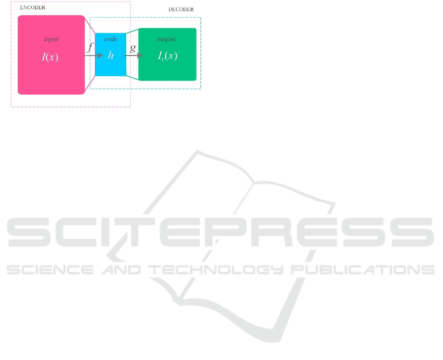
data means the images. As usual, AEs have a

symmetric three-tier input-code-output structure, as

shown in Figure 2, where the middle tier is for

encoding the input data. Pairs of adjacent tiers make

up two reciprocal components: input-code as an

encoder and code-output as a decoder (Goodfellow,

2016). The goal of AE is to restore the input data to

the output, while observing certain restrictions

imposed on the internal encoding. Because of these

restrictions, it is not allowed to simply copy data from

input to output. Typical restrictions are related to a

dimensionality reduction of intermediate (coding)

Figure 1: Representation of the “cameraman” image by

samples of random counts: A – the original image in TIF

format, B, C, D – sampling representations of the sizes,

respectively, 500 000, 1 000 000 and 5 000 000 counts.

data, which excludes input-output bijection. The

presence of such a bottleneck on the one hand and the

main AE task on the other hand implies some optimal

coding for intermediate data.

In the light of modern approaches, such a coding

can be synthesized basing on unsupervised AE

Generative Model for Autoencoders Learning by Image Sampling Representations

357

learning. Note that although the term "autoencoder"

is currently the most popular term, due to the very

broad scope of given definition, it can also be used

synonymously with auto-associative memory

networks (Kohonen, 1989), replicator ANN (Hecht-

Nielsen, 1995), etc.

Figure 2: Schema of a basic Autoencoder.

To formalize the AE problem, let us present its

general mathematical frame (Baldi, 2012). We

assume the following. First, the sets 𝒢 of images

𝐼𝑥⃗,𝑥⃗∈𝛺 and ℱ of internal images representations

(code) ℎ



⃗

are given (see Figure 2). Second, the classes

of operators 𝑓: 𝒢 → ℱ (encoders) and 𝑔: ℱ → 𝒢

(decoders), agreed in dimensions with ℱ and 𝒢 and

with the given restrictions are specified. Third, a

numerical measure of distortion between the image

𝐼𝑥⃗ and some of its reconstruction 𝐼



𝑥⃗ is available

– the so-called loss function 𝐿𝐼



𝑥⃗



,𝐼



𝑥⃗

(Goodfellow, 2016). Within this framework, the main

problem of AE is to minimize the loss function with

respect to the encoder 𝑓 and decoder 𝑔 operators:



𝑓

∗

,𝑔

∗



𝑎𝑟𝑔min

,

𝐿



𝐼



𝑥

⃗



, 𝑔 ∘

𝑓

𝐼



𝑥

⃗



(4)

Any solution 𝑓

∗

(5) would be considered as the

desired coding for the optimal restoration 𝑔

∗

of the

image. Unfortunately, solving (4) in its most general

form is an unrealistic task. Therefore, in the study of

practical problems, it is necessary to specify the

elements of the general AE framework. Different

kinds of AEs can be derived depending on the choice

of sets 𝒢 and ℱ, special classes of operators 𝑓 and 𝑔

and the explicit form of loss function 𝐿 . If, for

example, 𝒢 and ℱ are linear spaces of dimensions 𝑛

and 𝑝 respectively, 𝑓 and 𝑔 are appropriate linear

operators ( 𝑛  𝑝 and 𝑝  𝑛 matrixes) and 𝐿 is a

𝐿



norm

‖

𝐼



𝑥⃗



𝐼



𝑥⃗

‖



in 𝒢 , we get a linear

autoencoder. It is interesting to note that a linear

autoencoder results in the same internal data

representation ℎ



⃗

as the principal component analysis

(PCA) (Plaut, 2018). Moreover, it is easy to

generalize the PCA to nonlinear NLPCA, if weaken

the linearity condition for the encoder 𝑓: 𝒢 → ℱ.

Such (nonlinear) AEs can learn a non-linear

manifolds for coded data instead of finding a low

dimensional approximating hyperplane.

In our case, the images are specified by sampling

representations 𝑋







𝑥⃗





,𝑖  1,…,𝑘 , generated

according to the probability distribution density of the

counts 𝜌𝑥⃗|𝐼



𝑥⃗



, which is uniquely related to the

registered intensity 𝐼



𝑥⃗



(3). So, it is quite reasonable

to consider the set 𝒢 as the set of probability densities



𝜌



𝑥⃗





on the image surface 𝑥⃗∈𝛺. This immediately

brings us to the generative models for autoencoders

(Goodfellow, 2016). In contrast to the traditional AE,

which are most naturally interpreted as the

regularization schemes, autoencoders in generative

paradigm consider the internal encoded data ℎ



⃗

latent variables and the coding operation 𝑓: 𝒢 → ℱ as

inference procedure (computing latent representation

for given 𝑋



). In this regard, generative models learn

to maximize the likelihood of 𝐼



𝑥⃗



conditioned by

input data (representation) 𝑋



, rather than copying

inputs to outputs. So, regularization issues don't

matter much for generative AE. As an example, a

couple of generative modeling approaches to

autoencoders can be mentioned here – the variational

autoencoder (VA) (Kingma, 2014) and the generative

stochastic network (GSN) (Alain, 2015).

To formalize the generative model for sampling

representations 𝑋







𝑥⃗





, let us consider the first set

𝒢 as some parametric family 𝒢𝜌𝑥⃗ | 𝜃

⃗

, 𝑥⃗∈𝛺,

𝜃

⃗

∈𝛩⊂ℝ



of probability distribution densities of

individual count 𝑥⃗ . The parameters 𝜃

⃗

∈𝛩 of

representation are associated with the unknown

normalized intensity 𝐼



𝑥⃗



and are intended for its

parametric approximation. Parametrization of the

distributions under study 𝜌𝑥⃗|𝐼



𝑥⃗



 is a common

technique that simplifies the problem of functional

optimization to a problem of optimal parameters

estimation. The unsupervised learning for generative

model AE consists in fitting 𝜌𝑥⃗ | 𝜃

⃗

∗

∈𝒢 for some

𝜃

⃗

∗

, considering as AE output, to a training data 𝑋



Note, that formally, sampling representation 𝑋



is not

an element of 𝒢 and it can’t be considered as the input

of AE. Instead of it, we should utilize conditional

probability density 𝜌𝑥⃗ | 𝑋







𝑥⃗





. Assuming, in

the spirit of the Bayesian approach, that the

parameters 𝜃

⃗

are random variables with any prior

probability distribution density 𝑃𝜃

⃗

, similarly to

how it was done in (Antsiperov, 2021b), we can write

the following expression for the conditional density:

ICPRAM 2022 - 11th International Conference on Pattern Recognition Applications and Methods

358

𝜌𝑥

⃗

| 𝑋







𝑥

⃗













⃗

,

⃗



,...,

⃗











⃗



,...,

⃗







∬







⃗

,

⃗



,...,

⃗



|



⃗







⃗





⃗









⃗



,...,

⃗







∬







⃗

|



⃗











⃗





|



⃗







⃗





⃗









⃗



,...,

⃗







∬

𝜌𝑥

⃗

|𝜃

⃗

𝜌



𝜃

⃗

|𝑋







𝑥

⃗







𝑑𝜃

⃗



, (5)

where we used the property of the conditional iid of

all samples 𝑥⃗,𝑥⃗



,...,𝑥⃗



(for a given 𝜃

⃗

or, which is

the same, for a given 𝐼



𝑥⃗



). As it is known, density

𝜌



𝜃

⃗

|𝑋







𝑥⃗







is, at least asymptotically 𝑘≫1, a

much narrower function than 𝜌𝑥⃗|𝜃

⃗

 . Since the

maximum of 𝜌



𝜃

⃗

|𝑋







𝑥⃗







coincides with the

maximum likelihood estimate 𝜃

⃗



, the density

𝜌𝑥⃗|𝜃

⃗

 can be taken out from the integral in (5) as the

independent of 𝜃

⃗

factor 𝜌𝑥⃗|𝜃

⃗



. This immediately

leads to the following (see also (Antsiperov, 2021b)):

𝜌𝑥

⃗

| 𝑋







𝑥

⃗





≅𝜌𝑥

⃗

|𝜃

⃗



 .

(6)

Coming back, we can use at the input of AE the

density 𝜌𝑥⃗|𝜃

⃗



∈𝒢, which accumulates all the

necessary information of the representation 𝑋







𝑥⃗





by means of a statistic 𝜃

⃗



𝑥⃗



, that is a solution

of R.A. Fisher’s maximum likelihood equation

(Aldrich, 1997):

𝜃

⃗



𝑎𝑟𝑔max





⃗

∈

𝐿𝜃

⃗

;𝑋



,

𝐿𝜃

⃗

;𝑋



𝜌𝑋



| 𝜃

⃗



∏

𝜌𝑥

⃗



| 𝜃

⃗

 .





. (7)

Considering the developed generative model

formalization, it seems, that conceptually the solution

of the AE main problem becomes straightforward.

Namely, this solution consists in forming the density

𝜌𝑥⃗|𝜃

⃗



∈𝒢 at the input of the autoencoder, using

the sample representation 𝑋



(by generating sample

statistics 𝜃

⃗



𝑋



) and transmitting it in some coded

form to the output. Obviously, formed in such a

manner the input and output densities provide the

minimum for any suitable loss function

𝐿𝜌𝑥⃗|𝜃

⃗



,𝜌𝑥⃗ | 𝜃

⃗

∗

, if the appropriate encoding-

decoding procedures guarantee 𝜃

⃗

∗

~𝜃

⃗



The seeming elegance of solving AE problem

within the generative model framework is associated

with the replacement of the input data coding problem

by the problem of calculating maximum likelihood

estimate (7). However, the problem (7), which has

been known for a hundred years, starting with Fisher's

works (see (Aldrich, 1997)), in real applications turns

out not much simpler, than the coding problem.

Moreover, the development of such modern direction

as machine learning (including autoencoders) was

largely due to the needs of an approximate solution of

the maximum likelihood problem. For this reason, to

further refine the generative model, we will develop

the "proper autoencoder" method for solving the main

problem of the AE, considering it as a special class of

methods for solving the maximum likelihood

equation (7).

The main assumption for our special generative

model is that the parametric family 𝒢𝜌𝑥⃗ | 𝜃

⃗



admits latent (hidden) variables. Let us consider the

simplest case, where each count 𝑥⃗ is associated with

a single latent variable 𝑗, that takes only a finite set of

discrete values: 𝑗∈1,…,𝐾. Let us denote the

density of joint probability distribution of 𝑥⃗ and 𝑗 by

𝜌𝑥⃗,𝑗 | 𝜃

⃗

. In what follows, we implicitly assume that

𝜌𝑥⃗,𝑗 | 𝜃

⃗

 is more tractable than 𝜌𝑥⃗| 𝜃

⃗

, since the

latter is a marginal distribution of the former:

𝜌𝑥

⃗

|𝜃

⃗



∑

𝜌𝑥

⃗

𝑗

| 𝜃

⃗







(8)

and the sum in (8) can contain a large number 𝐾 of

terms. The density (9) is generally called the finite

mixture of components and traditionally components

are written in the form 𝜌𝑥⃗,𝑗 | 𝜃

⃗

𝑤



𝜌



𝑥⃗ | 𝜃

⃗

,

where 𝑤



 𝜌𝑗 | 𝜃

⃗

 is the weight (probability) of the

𝑗 –component, and 𝜌



𝑥⃗ | 𝜃

⃗

 is the conditional

distribution of the count coordinates 𝑥⃗ for the

component 𝑗 . As a rule, component weights are

considered as a subset of a parameters: 𝑤



⊂𝛩.

In accordance with (8), the density of the joint

distribution of the sampling representation 𝑋







𝑥⃗





(3) can be written in the form:

𝜌𝑋



|𝜃

⃗



∏



∑

𝜌𝑥

⃗



𝑗



| 𝜃

⃗

















∑



∏

𝜌𝑥

⃗



𝑗



|𝜃

⃗













⃗



∑

𝜌𝑋



,ℎ



⃗

| 𝜃

⃗







⃗

(9)

where the ordered set (vector) ℎ



⃗





𝑗



,…,𝑗





,𝑗



∈

1,…,𝐾 represents the latent variables of

autoencoder, i. e. the inner representation of

𝜌𝑋



| 𝜃

⃗

, defined on the 𝑛-cube ℱ1,…,𝐾



. It

is easy to see that the density (6) is also a finite

mixture of components with component weights

𝑊





⃗



∏

𝑤









and conditional distributions

𝜌





⃗

𝑋



| 𝜃

⃗



∏

𝜌





𝑥⃗



| 𝜃

⃗







of 𝑋



for given

component with multi-index ℎ



⃗

Generative Model for Autoencoders Learning by Image Sampling Representations

359

For densities representable in the form of mixtures

(9), there is an important relation between their so-

called score 𝑠⃗𝜃

⃗

,𝑋



∇





⃗

ln𝜌𝑋



| 𝜃

⃗

 and

corresponding scores for a joint distributions

𝑠⃗





⃗

𝜃

⃗

,𝑋



∇





⃗

ln𝜌𝑋



,ℎ



⃗

| 𝜃

⃗

:

𝑠⃗𝜃

⃗

,𝑋















| 



⃗



∇





⃗

𝜌𝑋



| 𝜃

⃗













| 



⃗



∑

∇





⃗

𝜌𝑋



,ℎ



⃗

| 𝜃

⃗







⃗



∑









,



⃗

| 



⃗











| 



⃗













,



⃗

| 



⃗



∇





⃗

𝜌𝑋



,ℎ



⃗

| 𝜃

⃗







⃗



∑

𝜌ℎ



⃗

|𝑋



,𝜃

⃗

𝑠

⃗





⃗

𝜃

⃗

,𝑋









⃗

(10)

The importance of scores in the statistics is

associated with the fact that sufficient conditions for

solution 𝜃

⃗



of the maximum likelihood problem (7)

can be written in the form: 𝑠⃗𝜃

⃗

,𝑋



0



⃗

Accordingly, the importance of the relation (10) lies

in the fact that it allows one to express these

conditions in an alternative form:

∑

𝜌ℎ



⃗

|𝑋



,𝜃

⃗

𝑠⃗





⃗

𝜃

⃗

,𝑋









⃗

0



⃗

(11)

Insofar as

𝑠⃗





⃗

𝜃

⃗

,𝑋



∇





⃗

ln𝜌 𝑋



,ℎ



⃗

| 𝜃

⃗



∑

∇





⃗

ln𝜌𝑥

⃗



𝑗



| 𝜃

⃗







. (12)

and if 𝜌𝑥⃗,𝑗 | 𝜃

⃗

 is more tractable than 𝜌𝑥⃗| 𝜃

⃗

 (8),

then the score 𝑠⃗





⃗

𝜃

⃗

,𝑋



 (12) will be more tractable

than 𝑠⃗𝜃

⃗

,𝑋



 and it turns out that the solution of (11)

is much easier to find than solution of 𝑠⃗𝜃

⃗

,𝑋0



⃗

In addition, it is easy to see that (11) is very

similar to the gradient optimization equations for the

well–known EM–algorithm (Gupta, 2010), or its hard

clustering variant, known as K–means segmentation.

Indeed, approximate solution of (11) can be carried

out by iterations containing two main steps. The first

step consists in calculating the latent variables ℎ



⃗

that

maximize the posterior distribution 𝜌ℎ



⃗

|𝑋



,𝜃

⃗



𝑋



,ℎ



⃗

| 𝜃

⃗

𝜌𝑋



| 𝜃

⃗

 for obtained in the previous

iteration parameters 𝜃

⃗

. And the second step is to find

a solution 𝜃

⃗

of the equation 𝑠⃗





⃗

𝜃

⃗

,𝑋



0



⃗

with ℎ



⃗

found at the first step.

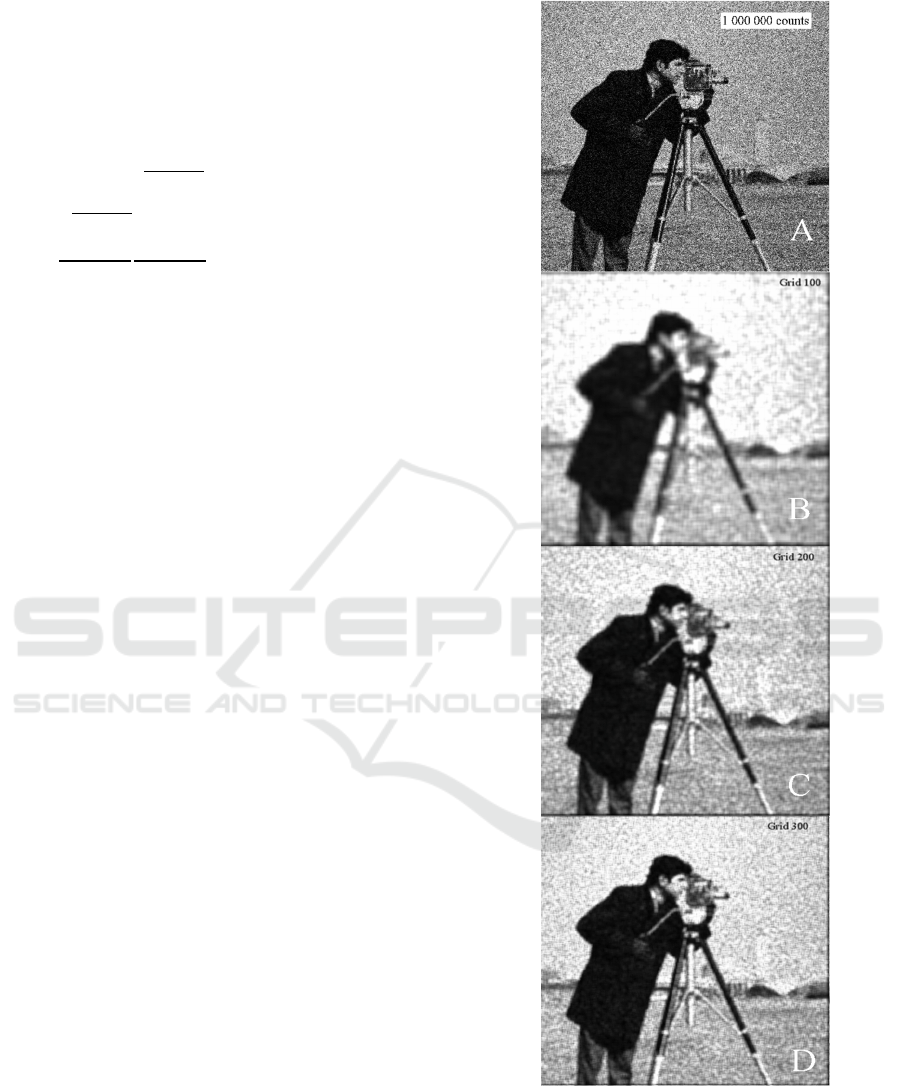
Figure 3: Reconstructions of “cameraman” image

(1 000 000 counts) by various number of components 𝐾 in

intermediate representation: A – the original image in TIF

format, B, C, D –reconstructions, corresponding to 𝐾 =

100

,250

, 300

components.

ICPRAM 2022 - 11th International Conference on Pattern Recognition Applications and Methods

360

Putting together all the conclusions obtained

above, the final encoding 𝑓 and decoding 𝑔 operators

of autoencoders in a generative model with latent

variables ℎ



⃗

(in a finite mixture model) can be

formulated as follows:

Encoding: 𝑓: 𝒢 → ℱ ∶ 𝜌 𝑋



| 𝜃

⃗

→ℎ



⃗

ℎ



⃗

𝑋



,𝜃

⃗



𝑎𝑟𝑔 max

∈



,…,





𝜌𝑥

⃗



𝑗

| 𝜃

⃗

,…,𝜌𝑥

⃗



𝑗

| 𝜃

⃗





. (13)

Decoding: 𝑔: ℱ → 𝒢 ∶ ℎ



⃗

→𝜌𝑋



| 𝜃

⃗

:

𝑠

⃗





⃗

𝜃

⃗

,𝑋



0



⃗

(14)

The developed approach to learning generative

autoencoders by image sampling representations can

be naturally implemented in the form of a recurrent

computational procedure. Some examples of

reconstruction of sampling representation shown in

Figure 1 C (1 000 000 counts) are shown in Figure 3.

4 CONCLUSIONS

In the framework of generative model, a new

approach is proposed It provides the synthesis of

learning methods for autoencoders by images,

presented as samples of random counts. The issues of

simplicity of interpretation of the approach and the

immediacy of its algorithmic implementation are the

main content of the work. They make it attractive in

both theoretical and practical terms, especially in the

context of modern machine learning-oriented trends.

In a sense, the proposed method is an adaptation of R.

Fisher's maximum likelihood method for

autoencoders, which is widely used in traditional

statistics. The fruitful use of the latter has led to a

huge number of important statistical results. In this

regard, the author expresses the hope that the

proposed approach will also be useful in solving a

wide range of modern machine learning problems.

REFERENCES

Alain, G., Bengio, Y., et. al. (2015). GSNs: Generative

Stochastic Networks. arXiv:1503.05571.

Aldrich, J. R.A. (1997). Fisher and the Making of

Maximum Likelihood 1912-1922. In Statistical

Science. V. 12(3). P. 162-176.

Antsiperov, V.E. (2021, a). Representation of Images by the

Optimal Lattice Partitions of Random Counts. In Pat.

Rec. and Image Analysis, V. 31(3), P. 381–393.

Antsiperov, V. (2021, b). New Maximum Similarity

Method for Object Identification in Photon Counting

Imaging. In Proc. of the 10th Int. Conf. ICPRAM 2021.

V. 1: ICPRAM, P. 341-348.

Baldi, P. (2012). Autoencoders, unsupervised learning, and

deep architectures. In Proc. of Machine Learning

Research, V. 27, PMLR, Bellevue, USA. P. 37–49.

Barber, D. (2012). Bayesian Reasoning and Machine

Learning. Cambridge Univ. Press, Cambridge.

Beghdadi, A., Larabi, M.C. Bouzerdoum, A.,

Iftekharuddin, K.M. (2013). A survey of perceptual

image processing methods. In Signal Processing: Image

Communication, V. 28(8) P. 811-831.

Fossum, E.R., Teranishi, N., et al. (eds.) (2017). Photon-

Counting Image Sensors. MDPI.

Fossum, E.R. (2020). The Invention of CMOS Image

Sensors: A Camera in Every Pocket. In Pan Pacific

Microelectronics Symposium. P. 1-6.

Fox, M. (2006). Quantum Optics: An Introduction. Oxford

University Press. Oxford, New York.

Gabriel, C.G., Perrinet L., et al. (eds.) (2015). Biologically

Inspired Computer Vision: Fundamentals and

Applications. Wiley-VCH, Weinheim.

Gallager, R. (2013). Stochastic Processes: Theory for

Applications. Cambridge University Press. Cambridge.

Goodfellow, I, Bengio, Y., Courville, A. (2016).

Autoencoders. In Deep Learning, MIT Press. P. 499.

Gupta, M. R. (2010). Theory and Use of the EM Algorithm.

In Foundations and Trends in Signal Processing, V.1

(3). P. 223-296.

Hecht-Nielsen, R. Replicator. (1995). Neural Networks for

Universal Optimal Source Coding. In SCIENCE, V.269

(5232). P. 1860-1863.

Hinton, G. E., Zemel, R. S. (1994). Autoencoders,

minimum description length and Helmholtz free

energy. In Adv. in neural inform. process V. 6. P. 3-10.

Kingma, D.P. (2014). Welling M. Auto-Encoding

Variational Bayes. arXiv:1312.6114.

Kohonen, T. (1989). Self-Organization and Associative

Memory, 3-d Edition. Springer.

Morimoto, K., Ardelean, A., et al. (2020) Megapixel time-

gated SPAD image sensor for 2D and 3D imaging

applications. In Optica V. 7(4). P. 346-354.

Murphy, K.P. (2012). Machine Learning: A Probabilistic

Perspective. MIT Press.

Pal, N.R. and Pal, S.K. (1991). Image model, Poisson

distribution and object extraction. In J. Pattern

Recognit. Artif. Intell. V. 5(3). P. 459–483.

Plaut, E. (2018). From Principal Subspaces to Principal

Components with Linear Autoencoders. arXiv:

1804.10253.

Rodieck, R.W. (1998). The First Steps in Seeing. Sinauer.

Sunderland, MA.

Seitz, P., Theuwissen, A.J.P. (eds). (2011). Single-photon

imaging. Springer. Berlin, New York.

Streit, R.L. (2010). Poisson Point Processes. Imaging,

Tracking and Sensing. Springer. New York.

Generative Model for Autoencoders Learning by Image Sampling Representations

361