
Melanoma Recognition
Michal Haindl
a
and Pavel
ˇ
Zid
b
The Institute of Information Theory and Automation, Czech Academy of Sciences,
Pod Vod
´
arenskou v
ˇ
e
ˇ
z
´
ı 4, Prague, Czech Republic
Keywords:
Skin Cancer Recognition, Melanoma Detection, Circular Markov Random Field Model.
Abstract:
Early and reliable melanoma detection is one of today’s significant challenges for dermatologists to allow
successful cancer treatment. This paper introduces multispectral rotationally invariant textural features of
the Markovian type applied to effective skin cancerous lesions classification. Presented texture features are
inferred from the descriptive multispectral circular wide-sense Markov model. Unlike the alternative texture-
based recognition methods, mainly using different discriminative textural descriptions, our textural representa-
tion is fully descriptive multispectral and rotationally invariant. The presented method achieves high accuracy
for skin lesion categorization. We tested our classifier on the open-source dermoscopic ISIC database, contain-
ing 23 901 benign or malignant lesions images, where the classifier outperformed several deep neural network
alternatives while using smaller training data.
1 INTRODUCTION
Diagnosing skin diseases is complicated. At least
3,000 identified varieties of skin diseases (Kawahara
and Hamarneh, 2019) with a prevalence that varies
by condition. Skin diagnosis is usually determined
using a biopsy, which, however lengthy, costly, un-
comfortable, and may introduce potential infectious
complications to the patient. Image-based automatic
skin diagnosis potentially avoids all these difficulties.
Automatic skin cancer recognition is a challenging
but proper application that can help dermatologists
in early cancer detection. Melanoma accounted for
41% skin-related deaths in the USA in 2013 (Kawa-
hara and Hamarneh, 2019) where every hour one per-
son dies from melanoma, while the highest melanoma
rate is in Australia (34 000 skin cancers every year)
and New Zealand (Zhang et al., 2020). Thus the early
melanoma diagnosis is of the utmost importance. Di-
agnosis of skin lesion type is a challenging task even
for a skilled dermatologist. The use of dermoscopy
imaging devices significantly improved the quality of
early melanoma detection. Further improvement is
possible by the use of computer-assisted diagnosis.
Automatic skin lesion categorization allows iden-
tification or learning of skin lesion types possible
without specific medical knowledge. Recent stud-
a
https://orcid.org/0000-0001-8159-3685
b
https://orcid.org/0000-0001-8249-1701
ies show that recognition systems can match or even
outperform clinicians in the diagnosis of individual
skin lesion images in controlled reader studies (Kawa-
hara and Hamarneh, 2019; Rotemberg et al., 2021).
Results comparison is difficult due to different data
sets or their subset used in different studies and of-
ten not appropriately described. (Ballerini et al.,
2013) reached 74% accuracy for five classes using
the hierarchical k-NN classifier using mean and co-
variance color matrices, and 12 features derived from
gray-level co-occurrence matrices (3888 features) on
their dataset with 960 images acquired from Canon
EOS 350D SLP camera. Authors (Gomez and Her-
rera, 2017) used an SVM classifier with histogram
and gray-level co-occurrence matrices-based features
and reached 70% accuracy on UDA, MSK, and
SONIC data sets. The gray level co-occurrence fea-
tures are similarly used as texture features in (Shak-
ourian Ghalejoogh et al., 2019).
Several algorithms (Akram et al., 2020; Ballerini
et al., 2013; Esteva et al., 2017; Favole et al., 2020;
Gessert et al., 2020; Hosny et al., 2020; Kawahara
et al., 2016; Khan et al., 2021; Mahbod et al., 2019;
Nida et al., 2019; Tschandl et al., 2019; Zhang et al.,
2019; Zhang et al., 2020) are using convolutional neu-
ral networks (CNN). (Kawahara et al., 2016) reached
85% accuracy for five classes on AlexNet (4096 fea-
tures) on the Dermofit (Ballerini et al., 2013) 1300 im-
ages. (Esteva et al., 2017) used GoogleNet Inception
722
Haindl, M. and Žid, P.
Melanoma Recognition.
DOI: 10.5220/0010936400003124
In Proceedings of the 17th International Joint Conference on Computer Vision, Imaging and Computer Graphics Theory and Applications (VISIGRAPP 2022) - Volume 4: VISAPP, pages
722-729
ISBN: 978-989-758-555-5; ISSN: 2184-4321
Copyright
c
2022 by SCITEPRESS – Science and Technology Publications, Lda. All rights reserved

v3 CNN and achieved 72% accuracy for three classes
and 55% accuracy for nine classes on 129450 images.
(Tschandl et al., 2019) use CNN for lesion segmen-
tation from the HAM10000 dataset (Tschandl et al.,
2018). (Zhang et al., 2019) used an attention resid-
ual learning convolutional neural network evaluated
on the ISIC-skin 2017 dataset (Codella et al., 2018)
with 87% accuracy for the melanoma classification.
We use the (ISI, ) skin image database chosen
by Favole et al. (Favole et al., 2020). The au-
thors (Favole et al., 2020) examine the performance
of AlexNet (Krizhevsky et al., 2012), Inception-
V1 (a.k.a. GoogLeNet) (Szegedy et al., 2015) and
Resnet50 (He et al., 2016) CNNs for the classifica-
tion problem of skin lesions.
Our study tests the circular 2D causal auto-
regressive adaptive random (2DSCAR) field model
and compares the results with results published in
(Favole et al., 2020). We use 23901 dermoscopic im-
ages of lesions from the ISIC image database. We
have chosen the 2018 JID Editorial, HAM10000,
MSK, SONIC, and UDA datasets. The presented
contribution is the accuracy improvement of skin
melanoma recognition while using a smaller training
set and faster learning than the alternative deep neural
net approach.
2 CIRCULAR MARKOVIAN
TEXTURE REPRESENTATION
Figure 1: The octagonal, circular path. The numbers mark
the site order in which the pixels s, i.e., I
cs
s
contextual
neighborhoods are traversed. Furthermore, the center pixel
r, for which the statistics are computed, is marked as the
yellow square.
The circular 2D causal auto-regressive adaptive ran-
dom (2DSCAR) field model (Fig. 1) is a generaliza-
tion of the directional 2DCAR model (Haindl, 2012)
to the rotationally invariant form, which was intro-
duced in (Reme
ˇ
s and Haindl, 2018) for bark classifi-
cation application. The model’s contextual neighbor
index shift set denoted I
cs
r
is functional. The model
for d spectral bands can be defined in the following
matrix form:
Y
r
= γZ
r
+ e
r
, (1)
where γ = [A
1
, . . . , A
η
] is the parameter matrix, A
i
=
diag[a
i1
, . . . , a
id
] ∀i, a
i j
are unknown parameters to
be estimated (2), η = cardinality(I
cs
r
), r = [r
1
, r
2
] is
spatial multi-index (r
1
row and r
2
column indices) de-
noting history of movements on the lattice I, e
r
de-
notes the driving white Gaussian noise vector with
zero mean and a constant but unknown covariance
matrix Σ, and Z
r
is a neighborhood support vec-
tor of multispectral pixels Y
r−s
where s ∈ I
cs
r
.
All 2DSCAR model statistics can be efficiently
analytically estimated as proven in (Haindl, 2012).
The Bayesian parameter estimation (conditional mean
value)
ˆ
γ can be accomplished using fast, numerically
robust and recursive statistics (Haindl, 2012), given
the known 2DSCAR process history
Y
(t−1)
= {Y
t−1
, Y
t−2
, . . . , Y
1
, Z
t
, Z
t−1
, . . . , Z
1
} :
ˆ
γ
T
t−1
= V
−1
zz(t−1)
V
zy(t−1)
, (2)
V
t−1
=
˜
V
t−1
+V
0
, (3)
˜
V
t−1
=
∑
t−1
u=1
Y
u
Y
T
u
∑
t−1
u=1
Y
u
Z
T
u
∑
t−1
u=1
Z
u
Y
T
u
∑
t−1
u=1
Z
u
Z
T
u
=
˜
V
yy(t−1)
˜
V
T
zy(t−1)
˜
V
zy(t−1)
˜
V
zz(t−1)
, (4)
where V
t−1
is the data gathering matrix, V
0
is
a positive definite initialization matrix (see (Haindl,
2012)). We introduce a new octagonal traversing or-
der multi-index t of the sequence of multi-indices r,
to simplify notation, which depends on the selected
model movement in the underlying lattice I (e.g.,
T = {t
1
, t
1
+(1; 0), t
1
+(2; 0), . . . , t
16
+(−1; −1)} for
Fig. 1). The optimal functional causal contextual
neighbourhood I
cs
r
(Fig. 2) can be solved analytically
by a straightforward generalization of the Bayesian
estimate derived in (Haindl, 2012). We did not opti-
mize the neighbourhood I
cs
r
but used its fixed form
Fig. 2 to simplify and speed up our experiments.
However, if this neighborhood is optimized, we can
expect further accuracy improvement. The model can
be easily applied also to various synthesis and restora-
tion applications. The 2DSCAR model pixel-wise
synthesis is a direct application of the equation (1)
fed from a Gaussian noise generator for any 2DSCAR
model.
2.1 Circular Models
The 2DSCAR model moves (r) on the circular path
on the lattice I as is illustrated in Fig. 1. The causal
Melanoma Recognition
723

→ ↓
· · · • · ·
· • · · · ·
· · • · · ·
· · · · · ·
• · · · · •
· · · · • r
· • · · · ·
· · · · • ·
· · · • · ·
· · · · · •
• · · · · ·
r • · · · ·
← ↑
r • · · · ·
• • · · · •
· · · · · ·
· · · • · ·
· · · · • ·
· · • · · ·
· · · · • r
· · · · · •
• · · · · ·
· · • · · ·
· • · · · ·
· · · · • ·
Figure 2: The applied fixed causal functional contextual
neighbourhood I
cs
r
in four selected directions, • are the con-
textual neighbours, r is the neigbourhood location index.
Upper left: rightwards (Fig.1-13,14,15), upper right: down-
wards (Fig.1-1,2,3), bottom left leftwards (Fig.1-5,6,7), bot-
tom right upwards (Fig.1-9,10,11), respectively.
neighborhood I
c
r
has to be transformed to be con-
sistent for each direction in the traversed path, as de-
noted in Fig. 2. The paths used can be arbitrary as
long as they keep transforming the causal neighbor-
hood into I
cs
r
in such a way that the model has vis-
ited all neighbors of a control pixel r. Thus these
neighbors are known from the previous steps. We
shall call all these causal paths as circulars further on.
In this paper, we present the octagonal type of path
- (Fig. 1). However, alternatively, a circular path can
be used as well. The parameters for the center pixel
(the yellow square in Fig. 1) of the circular are esti-
mated after the whole path is completed. Since this
model’s equations do not need the whole history of
movement through the image but only the local neigh-
borhood of a single circular, the 2DSCAR models can
be easily parallelized. This memory restriction is ad-
vantageous in comparison to the standard directional
CAR models (Haindl, 2012). The 2DSCAR models
exhibit rotational invariant properties for the circular
shape paths, thanks to the CAR model’s memory of
all the visited pixels. Additional prior contextual in-
formation can be easily incorporated if every initial-
ization matrix V
0
= V
t−1
, for example, this matrix can
be initialized from the previous data gathering matrix.
2.2 Multispectral Rotationally
Invariant Features
We analyzed the 2DSCAR model around all pixels
with the vertical and horizontal stride of 2 to speed
up the computation for feature extraction. The fol-
lowing α
1
, α
2
, α
3
illumination invariant features ini-
tially derived for the 3DCAR model (Haindl, 2012)
were adapted for the 2DSCAR model:
α
1
= 1 + Z
T
r
V
−1
zz
Z
r
, (5)
α
2
=
r
∑
r
(Y
r
−
ˆ
γZ
r
)
T
λ
−1
r
(Y
r
−
ˆ
γZ
r
) , (6)
α
3
=
r
∑
r
(Y
r
− µ)
T
λ
−1
r
(Y
r
− µ) , (7)
where µ is the mean value of vector Y
r
and
λ
t−1
= V
yy(t−1)
−V
T
zy(t−1)
V
−1
zz(t−1)
. (8)
The inversion data gathering matrix V
−1
zz(t−1)
is up-
dated in its square-root Cholesky factor to guaran-
tee numerical stability for computed model statistics
(Haindl, 2012). Additional used texture features are
also the estimated trace of γ parameters, the poste-
rior probability density (Haindl, 2012)
p(Y
r
|Y
(r−1)
,
ˆ
γ
r−1
) = (9)
Γ(
β(r)−η+3
2
)
Γ(
β(r)−η+2
2
) π
1
2
|λ
(r−1)
|
1
2
(1 + X
T
r
V
−1
x(r−1)
X
r
)
1
2
1 +
(Y
r
−
ˆ
γ
r−1
X
r
)
T
λ
−1
(r−1)
(Y
r
−
ˆ
γ
r−1
X
r
)
1 + X
T
r
V
−1
x(r−1)
X
r
!
−
β(r)−η+3
2
,
β(r) = r + η − 2, and the absolute error of the one-
step-ahead model prediction (Haindl, 2012):
Abs(GE) =
E
n
Y
r
|Y
(r−1)
o
−Y
r
=
|
Y
r
−
ˆ
γ
r−1
X
r
|
. (10)
Fig. 3 illustrates 15 selected features computed from
the HAM database ISIC 0024313 malignant lesion.
3 SKIN LESION CLASSIFIER
The algorithm starts with image subsampling to the
width of 512 px (for larger images) while keeping the
aspect ratio to speed up the feature extraction part.
This subsampling ratio depends on application data;
it is a compromise between the algorithm efficiency
and its recognition rate. Every pixel has extracted fea-
tures θ, as described in Sec. 2. The resulting feature
space indexed on the lattice I is assumed to be gov-
erned by the multivariate Gaussian distribution. The
n estimated Gaussian parameters then represent every
training image sample:
VISAPP 2022 - 17th International Conference on Computer Vision Theory and Applications
724
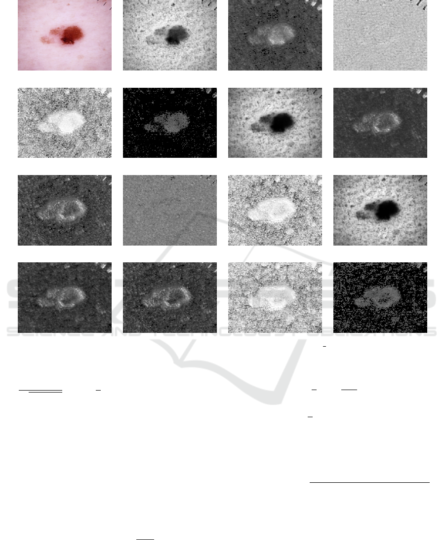
HAM source feature 1 feature 2 feature 4
feature 10 feature 11 feature 12 feature 13
feature 14 feature 18 feature 21 feature 23
feature 24 feature 25 feature 32 feature 33
Figure 3: Examples of the selected 2DSCAR features computed from the HAM ISIC 0024313 malignant texture.
N (θ|µ, Σ) = (11)
1
p
(2π)
n
|Σ|
exp
−
1
2
(θ − µ)
T
Σ
−1
(θ − µ)
.
In the classification step, the Gaussian distribu-
tion parameters are estimated for the classified im-
age in the same way. The classified image parame-
ters are then compared with all the distributions from
the training samples set using the 1 nearest-neighbor
classifier (1-NN) and the Jeffreys divergence (14) as
the measure. The KL divergence is a probability dis-
tribution non-symmetric similarity measure between
two distributions; it is defined as:
D( f (x)||g(x))
de f
=
Z
f (x)log
f (x)
g(x)
dx , (12)
where f (x), g(x are the compared probability densi-
ties.
The KL divergence for the Gaussian distribution
data model can be solved analytically:
D( f (x)||g(x)) =
1
2
log
|Σ
g
|
|Σ
f
|
+tr(Σ
−1
g
Σ
f
) − d
+
1
2
µ
f
− µ
g
)
T
Σ
−1
g
(µ
f
− µ
g
. (13)
We use the Jeffreys divergence, which the sym-
metrized variant of the Kullback-Leibler divergence:
D
s
( f (x)||g(x)) =
D( f (x)||g(x)) + D(g(x)|| f (x))
2
.
(14)
The selected class is the class of a training image
with the lowest Jeffreys divergence from the tested
image. The primary benefit of our method is the sig-
nificant compression of the training database into the
Gaussian distribution parameters (as we extract only
about n = 40 features, depending on the chosen
neighborhood, we need to store 40 real numbers for
the mean and 40×40 numbers for the covariance ma-
trix). The subsequent comparison with the training
Melanoma Recognition
725
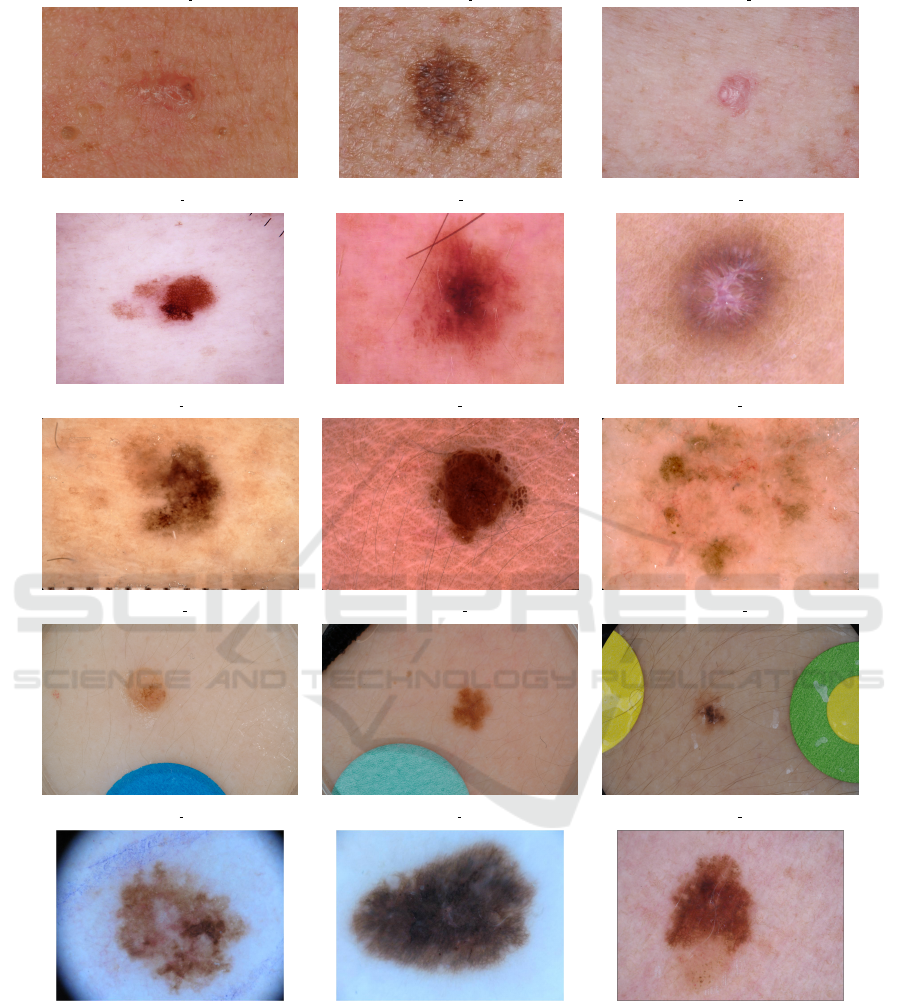
2018 JID m (ISIC 0024233) 2018 JID m (ISIC 0024284) 2018 JID u (ISIC 0024209)
HAM m (ISIC 0024313) HAM b (ISIC 0024306) HAM u (ISIC 0024318)
MSK m (ISIC 0011460) MSK b (ISIC 0011409) MSK u (ISIC 0011444)
SONIC b (ISIC 0000579) SONIC b (ISIC 0000557) SONIC b (ISIC 0003588)
UDA m (ISIC 0000002) UDA b (ISIC 0000000) UDA b (ISIC 0000020)
Figure 4: Examples of skin lesion images (m - malignant, b - benign, u - unknown) from the used datasets.
database is thus extremely fast, enabling us to com-
pare hundreds of thousands of image feature distribu-
tions per second on an ordinary computer.
4 EXPERIMENTAL SKIN DATA
We verified the proposed method on the publicly
available skin image International Skin Imaging Col-
laboration Archive (ISIC) database (ISI, ; Rotemberg
et al., 2021). We used the following datasets from the
VISAPP 2022 - 17th International Conference on Computer Vision Theory and Applications
726
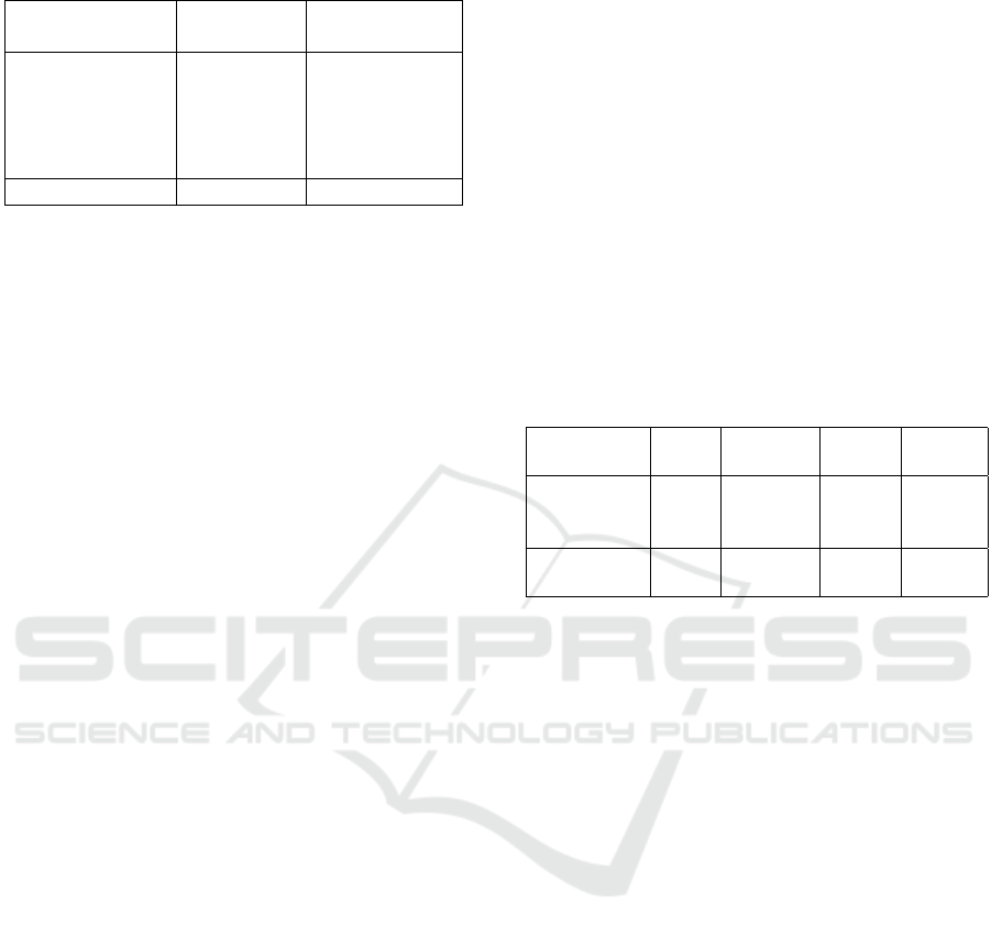
Table 1: Used datasets.
Dataset No. of images Image resolution
[pixels]
2018 JID Editorial 100 various
HAM10000 10 015 600 × 450
MSK 3 918 various
SONIC 9 251 3024 × 2016
UDA 617 various
total 23 901
ISIC archive (Tab. 1) to be able to compare our results
with the results published in (Favole et al., 2020):
The 2018 JID Editorial dataset contains selected
100 sequentially biopsied cutaneous melanomas (37),
basal cell carcinomas (40), and squamous cell
carcinomas (23) with high-quality clinical images
(Navarrete-Dechent et al., 2018) from the ISIC
archive. All lesions originated from Caucasian pa-
tients in the southern United States. Each lesion in
the skin datasets is represented by a single image in
the JPEG format.
The HAM10000 dataset (Tschandl et al., 2018) is
made up of 10 015 images and was collected over 20
years. Thus, the older images were digitized from
slides with a Nikon Coolscan 5000 ED scanner in
300 DPI resolution. The more recent images were
acquired from the digital dermatoscopy system Mole-
Max HD or the DermLiteTM Foto camera.
The MSK dataset (Codella et al., 2018) which
contains five subsets made up of 3918 in total. This
set with 3 to 5 images per lesion was acquired using
a dermoscopic attachment to either a digital single re-
flex lens (SLR) camera or a smartphone (Rotemberg
et al., 2021).
The SONIC dataset (Gomez and Herrera, 2017)
contains 9251 images from SONIC Healthcare, Aus-
tralia, which is acquired with Fujifilm FinePix S2 Pro
and 176 Nikon D300 cameras.
The UDA dataset contains two subsets which are
made up of 617 images. It includes melanoma and
benign lesions with a histopathological diagnosis or
clinically benign history containing metadata with pa-
tient age, diagnosis, gender, and anatomic location.
The ISIC data is highly unbalanced, with 80% be-
nign, 10% malignant, and 10% unknown images, this
severe underrepresentation of the most common skin
lesions can lead to a much lower diagnostic accuracy
when many samples are wrongly assigned to the same
class. Authors (Favole et al., 2020) tried to prevent
this problem by adding an altered version of malig-
nant and unknown images. We did not use such help
to see if our features can outperform the deep neural
net results even with a much smaller learning data set.
Fig. 4 illustrates the malignant, benign, or un-
known image examples of all five datasets. We have
used the leave-one-out approach for the classification
rate estimation and only on the original dataset with-
out any data augmentation as was done in the com-
pared deep neural net results (Favole et al., 2020).
Although in (Favole et al., 2020) the ratio of training
and testing sets is 80:20, due to the data augmenta-
tion, they still use the double size training set than the
presented method. Thus both validation approaches
(hold-out and leave-one-out) can be compared. The
augmented data in their validation set ((Favole et al.,
2020)) artificially increased their accuracy. Thus our
improvement in Tab. 3 would be in the correct com-
parison even higher.
Table 2: The 2DSCAR method results for used skin
datasets.
Benign Malignant Unknow Precision
gr. truth gr. truth gr. truth [%]
Benign int. 17941 858 454 93.2
Malignant int. 965 1175 279 48.6
Unknown int. 467 252 1510 67.7
Sensitivity Accuracy
[%] 92.6 51.4 67.3 86.3
5 RESULTS
Our experiment compares three separate lesion
classes - benign, malignant, and unknown images us-
ing a single resolution level. We have reached 86.3%
accuracy on the selected dataset. The sensitivity for
all classes is between 51.4 − 92.6 [%] with median
value 67.3% and precision 48.6 − 93.2 [%] with me-
dian value 67.7%. More details about the results are
in Tab. 2. If we added all flipped versions of malig-
nant and unknown images as in (Favole et al., 2020),
the test database would contain 52% benign, 24% ma-
lignant, and 24% unknown images, and the total num-
ber of images in the test database is 37485. The ac-
curacy would be improved to 95% and significantly
in malignant (precision 94%, sensitivity 99.7%) and
unknown images (precision 88%, sensitivity 99.7%).
We compared the accuracy results of the 2DSCAR
with the three CNNs evaluated in (Favole et al., 2020)
and additional three recently published CNN meth-
ods. The comparative results are in Tab. 3 with
each method’s number of parameters. The presented
method has three order fewer parameters than the al-
ternative CNNs, which means that our method needs
much less data for our reliable model learning. The
training times reported in (Favole et al., 2020) are be-
tween 47 minutes for the fastest Inception-V1 until 72
Melanoma Recognition
727
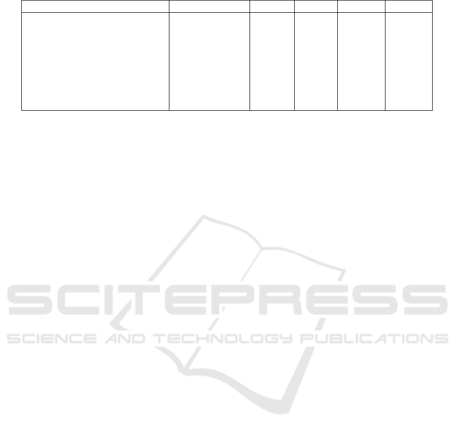
Table 3: Accuracy comparison. Results denoted
∗
use pre-trained nets with transfer learning.
Method No. of parameters Accuracy Precision Sensitivity Specificity
2DSCAR 1.6 · 10
3
0.86 0.70 0.71 0.87
2DSCAR augmented 1.6 · 10
3
0.95 0.94 0.97 0.98
AlexNet (Favole et al., 2020) 6 · 10
7
0.74 - - -
Inception-V1 (Favole et al., 2020) 5 · 10
6
0.70 - - -
RestNet50 (Favole et al., 2020) 2.6 · 10
7
0.74 - 0.75 0.86
ARL-CNN50
∗
(Zhang et al., 2019) 2.3 · 10
7
0.86 - 0.77 0.88
R-CNN
∗
(Khan et al., 2021) 2.3 · 10
7
0.86 0.87 0.86 -
Hosny
∗
(Hosny et al., 2020) 5 · 10
6
0.98 - 0.98 0.99
minutes for RestNet50. We list the results of the last
three methods (
∗
) for broad outline only. These meth-
ods cannot be directly compared because their authors
do not specify their training data and other parameters
precisely.
Although we eliminated variable illumination and
the observation rotation problem using the illumina-
tion and rotationally invariant features in our study,
other challenges, such as viewing angles, body posi-
tion, observation distance, resolution, or variability in
acquisition technologies, need to be treated for reli-
able and fully automatic skin diagnosis system. We
plan to investigate these research problems in our fu-
ture studies.
6 CONCLUSION
We present the method for lesion image catego-
rization. The classifier uses rotationally invariant
monospectral Markovian textural features from all
three spectral classes. Our textural features are analyt-
ically derived from the underlying descriptive textural
model and can be efficiently, recursively, and adap-
tively learned. Our 2DSCAR features are rotationally
invariant, exploit information from all spectral bands,
and can be easily parallelized or made fully illumi-
nation invariant if the non-illumination invariant fea-
tures are excluded (the posterior probability density
and the absolute error of the one-step-ahead predic-
tion). The classifier does not need extensive learn-
ing data contrary to the convolutional neural nets and
outperforms in classification accuracy three deep net-
work nets on the same data set with more than 12%.
If we add flipped versions of the malignant and un-
known images for learning as was done with the al-
ternative three deep network nets, we could outper-
form these methods up to 20%. Another benefit of
the presented method is the order of magnitude faster
learning.
ACKNOWLEDGMENT
The Czech Science Foundation project GA
ˇ
CR 19-
12340S supported this research.
REFERENCES
Isic - the international skin imaging collaboration, univer-
sity dermatology center.
Akram, T., Lodhi, H. M. J., Naqvi, S. R., Naeem, S., Al-
haisoni, M., Ali, M., Haider, S. A., and Qadri, N. N.
(2020). A multilevel features selection framework for
skin lesion classification. Human-centric Computing
and Information Sciences, 10(1):1–26.
Ballerini, L., Fisher, R. B., Aldridge, B., and Rees, J.
(2013). A color and texture based hierarchical k-nn
approach to the classification of non-melanoma skin
lesions. In Color Medical Image Analysis, pages 63–
86. Springer.
Codella, N. C., Gutman, D., Celebi, M. E., Helba, B.,
Marchetti, M. A., Dusza, S. W., Kalloo, A., Liopy-
ris, K., Mishra, N., Kittler, H., et al. (2018). Skin
lesion analysis toward melanoma detection: A chal-
lenge at the 2017 international symposium on biomed-
ical imaging (isbi), hosted by the international skin
imaging collaboration (isic). In 2018 IEEE 15th In-
ternational Symposium on Biomedical Imaging (ISBI
2018), pages 168–172. IEEE.
Esteva, A., Kuprel, B., Novoa, R. A., Ko, J., Swetter, S. M.,
Blau, H. M., and Thrun, S. (2017). Dermatologist-
level classification of skin cancer with deep neural net-
works. Nature, 542:115–118.
Favole, F., Trocan, M., and Yilmaz, E. (2020). Melanoma
detection using deep learning. In International
Conference on Computational Collective Intelligence,
pages 816–824. Springer.
Gessert, N., Nielsen, M., Shaikh, M., Werner, R., and
Schlaefer, A. (2020). Skin lesion classification using
ensembles of multi-resolution efficientnets with meta
data. MethodsX, 7:100864.
Gomez, C. and Herrera, D. S. (2017). Recognition of skin
melanoma through dermoscopic image analysis . In
Romero, E., Lepore, N., Brieva, J., and Garca, J. D.,
VISAPP 2022 - 17th International Conference on Computer Vision Theory and Applications
728

editors, 13th International Conference on Medical In-
formation Processing and Analysis, volume 10572,
pages 326 – 336. Int. Society for Optics and Photon-
ics, SPIE.
Haindl, M. (2012). Visual data recognition and model-
ing based on local markovian models. In Florack,
L., Duits, R., Jongbloed, G., Lieshout, M.-C., and
Davies, L., editors, Mathematical Methods for Signal
and Image Analysis and Representation, volume 41
of Computational Imaging and Vision, chapter 14,
pages 241–259. Springer London. 10.1007/978-1-
4471-2353-8 14.
He, K., Zhang, X., Ren, S., and Sun, J. (2016). Deep resid-
ual learning for image recognition. In Proceedings of
the IEEE conference on computer vision and pattern
recognition, pages 770–778.
Hosny, K. M., Kassem, M. A., and Foaud, M. M. (2020).
Skin melanoma classification using roi and data aug-
mentation with deep convolutional neural networks.
Multimedia Tools and Applications, 79(33):24029–
24055.
Kawahara, J., BenTaieb, A., and Hamarneh, G. (2016).
Deep features to classify skin lesions. In 2016 IEEE
13th International Symposium on Biomedical Imaging
(ISBI), pages 1397–1400. IEEE.
Kawahara, J. and Hamarneh, G. (2019). Visual diagnosis of
dermatological disorders: Human and machine per-
formance.
Khan, M. A., Zhang, Y.-D., Sharif, M., and Akram,
T. (2021). Pixels to classes: intelligent learning
framework for multiclass skin lesion localization and
classification. Computers & Electrical Engineering,
90:106956.
Krizhevsky, A., Sutskever, I., and Hinton, G. E. (2012). Im-
agenet classification with deep convolutional neural
networks. In Advances in neural information process-
ing systems, volume 25, pages 1097–1105.
Mahbod, A., Schaefer, G., Ellinger, I., Ecker, R., Pitiot, A.,
and Wang, C. (2019). Fusing fine-tuned deep features
for skin lesion classification. Computerized Medical
Imaging and Graphics, 71:19–29.
Navarrete-Dechent, C., Dusza, S. W., Liopyris, K.,
Marghoob, A. A., Halpern, A. C., and Marchetti,
M. A. (2018). Automated dermatological diagnosis:
hype or reality? The Journal of investigative derma-
tology, 138(10):2277.
Nida, N., Irtaza, A., Javed, A., Yousaf, M. H., and Mah-
mood, M. T. (2019). Melanoma lesion detection and
segmentation using deep region based convolutional
neural network and fuzzy c-means clustering. Inter-
national journal of medical informatics, 124:37–48.
Reme
ˇ
s, V. and Haindl, M. (2018). Rotationally invariant
bark recognition. In X., B., E., H., T., H., R., W., B.,
B., and A., R.-K., editors, IAPR Joint International
Workshop on Statistical Techniques in Pattern Recog-
nition and Structural and Syntactic Pattern Recogni-
tion (S+SSPR 2018), volume 11004 of Lecture Notes
in Computer Science, pages 22 – 31. Springer Nature
Switzerland AG.
Rotemberg, V., Kurtansky, N., Betz-Stablein, B., Caffery,
L., Chousakos, E., Codella, N., Combalia, M., Dusza,
S., Guitera, P., Gutman, D., et al. (2021). A patient-
centric dataset of images and metadata for identify-
ing melanomas using clinical context. Scientific data,
8(1):1–8.
Shakourian Ghalejoogh, G., Montazery Kordy, H., and
Ebrahimi, F. (2019). A hierarchical structure based on
stacking approach for skin lesion classification. Ex-
pert Systems with Applications, 145:113127.
Szegedy, C., Liu, W., Jia, Y., Sermanet, P., Reed, S.,
Anguelov, D., Erhan, D., Vanhoucke, V., and Rabi-
novich, A. (2015). Going deeper with convolutions.
In Proceeding of the IEEE conference on computer
vision and pattern recognition, pages 1–9.
Tschandl, P., Rosendahl, C., and Kittler, H. (2018). The
ham10000 dataset, a large collection of multi-source
dermatoscopic images of common pigmented skin le-
sions. Scientific data, 5(1):1–9.
Tschandl, P., Sinz, C., and Kittler, H. (2019). Domain-
specific classification-pretrained fully convolutional
network encoders for skin lesion segmentation. Com-
puters in biology and medicine, 104:111–116.
Zhang, J., Xie, Y., Xia, Y., and Shen, C. (2019). Attention
residual learning for skin lesion classification. IEEE
transactions on medical imaging, 38(9):2092–2103.
Zhang, N., Cai, Y.-X., Wang, Y.-Y., Tian, Y.-T., Wang, X.-
L., and Badami, B. (2020). Skin cancer diagnosis
based on optimized convolutional neural network. Ar-
tificial intelligence in medicine, 102:101756.
Melanoma Recognition
729
