
On Finding k Earliest Arrival Time Journeys in Public Transit Networks
Ali Al-Zoobi
1
, David Coudert
1
, Arthur Finkelstein
2
and Jean-Charles R
´
egin
1
1
Universit
´
e C
ˆ
ote d’Azur, Inria, CNRS, I3S, Sophia Antipolis, France
2
Instant System, Sophia Antipolis, France
fi
Keywords:
Public Transit Routing, Shortest Path, Dissimilar Paths.
Abstract:
Journey planning in (schedule-based) public transit networks has attracted interest from researchers in the last
decade. In particular, many algorithms aiming at efficiently answering queries of journey planning have been
proposed. However, most of the proposed methods give the user a single or a limited number of journeys in
practice, which is undesirable in a transportation context. In this paper, we consider the problem of finding
k earliest arrival time journeys in public transit networks from a given origin to a given destination, i.e., an
earliest arrival journey from the origin to the destination, a second earliest arrival journey, etc. until the k
th
earliest arrival journey. For this purpose, we propose an algorithm, denoted by Yen - Public Transit (Y-PT),
which extends to public transit networks the algorithm proposed by Yen to find the top-k shortest simple paths
in a graph. Moreover, we propose a more refined algorithm, called Postponed Yen - Public Transit (PY-PT),
enabling a considerable speed up in practice. Our experiments on several public transit networks show that, in
practice, PY-PT is faster than Y-PT by an order of magnitude.
1 INTRODUCTION
In the context of multimodal transportation, journey
planning in (schedule-based) public transit networks
and accelerating queries for efficient journey planning
is a long-standing problem (Bast et al., 2016). In the
last decade, many algorithms have been developed
not only to efficiently answer basic queries like the
quickest or the earliest arrival journey, but also to op-
timize additional criteria like the number of transfers,
the cost of the trip, etc. or even to offer Pareto optimal
solutions combining several criteria (Bast et al., 2016;
Delling et al., 2015; Dibbelt et al., 2018).
A transit network is a set of stops (such as bus
stops or train stations), a set of routes (such as bus,
tramways, ferries, metro or train lines), and a set of
trips. Trips correspond to individual vehicles that visit
the stops along a certain route at a specific time of the
day. Trips can be further subdivided into sequences of
elementary connections, each given as a pair of (ori-
gin/destination) stops and (departure/arrival) times
between which the vehicle travels without stopping.
In addition, footpaths model walking transfers be-
tween nearby stops. A journey is a sequence of trips
one can take within a transit network (also referred to
as a transportation network or a timetable).
The k Shortest Simple Paths Problem. A directed
graph (digraph for short) is a set of vertices connected
by arcs. A path from a source to a destination in
a digraph is a sequence of vertices starting from the
source and ending at the destination, such that con-
secutive vertices are connected by an arc. A path is
simple if it has no repeated vertices. The length (or
weight or cost) of a path is the sum of the lengths
(or weights or costs) of its arcs. In this context, the
k shortest simple paths (kSSP) problem asks to find
a set S of k distinct simple paths from a source to a
destination such that no path outside S has a length
strictly lower than any path in S. This problem can
be solved in time O(kn(m + nlogn)) using the algo-
rithm proposed by Yen (Yen, 1971), where n is the
number of vertices and m is the number of arcs. Since
this is the best known time complexity for this prob-
lem, a significant research effort has been put on the
design of algorithms for efficiently solving the kSSP
problem in practice (Kurz and Mutzel, 2016; Al Zoobi
et al., 2020; Al Zoobi et al., 2021a). Note that, if the
paths of S are not required to be simple, the prob-
lem can be solved by Eppstein’s algorithm in time
O(k + m + n log n) (Eppstein, 1998).
In fact, a road network can be modelled using a
weighted directed graph where crossroads are repre-
sented by vertices and routes by arcs with length cor-
responding to the distances or the travel time between
314
Al-Zoobi, A., Coudert, D., Finkelstein, A. and Régin, J.
On Finding k Earliest Arrival Time Journeys in Public Transit Networks.
DOI: 10.5220/0010977200003117
In Proceedings of the 11th International Conference on Operations Research and Enterprise Systems (ICORES 2022), pages 314-325
ISBN: 978-989-758-548-7; ISSN: 2184-4372
Copyright
c
2022 by SCITEPRESS – Science and Technology Publications, Lda. All rights reserved

crossroads. So, finding k “best” (shortest, fastest or
cheapest) paths from a given origin to a given des-
tination in a road network is straightforward using
any kSSP algorithm. Unfortunately, this problem be-
comes harder in public transit networks. First, be-
cause public transit networks are time dependent, i.e.,
certain segments of the network can only be traversed
at specific times. Second, several additional optimiza-
tion criteria are considered in public transit network
such as the arrival time, the departure time, the num-
ber of transfers, etc.
Journey Planning Queries in Public Transit Net-
works. A plethora of algorithms were proposed to
efficiently answer queries of optimal journeys from a
given origin o to a given destination d after a depar-
ture time t
0
in a public transit network. For instance,
the Connection Scan Algorithm (CSA) (Dibbelt et al.,
2018) is the fastest algorithm, without any prepro-
cessing routine, enabling to find an earliest arrival
journey from o to d departing after t
0
. With the
help of a heavy preprocessing routine, the Transfer
Patterns algorithm (Bast et al., 2010) can achieve a
tremendous speed up with respect to the CSA. Be-
sides, Round Based Public Transit Routing (RAP-
TOR) (Delling et al., 2015) is the fastest algorithm
(also without any preprocessing routine) enabling to
compute a Pareto optimal set of journeys optimizing
the arrival time and the number of transfers of a jour-
ney. Recently, Bast et al. (Bast et al., 2016) presented
an extensive survey on the topic of journey planning
in road and public transit networks.
Related Work. Vo et al. (Vo et al., 2015) proposed a
time dependent graph modeling a bus network. Then,
they adapt Yen’s algorithm to find alternative journeys
in this network model. Precisely, they select a set of
alternative journeys (journeys sharing only a limited
part of their common edges) among those given by
Yen’s adaptation.
As shown below, Yen’s algorithm uses Dijkstra’s
algorithm as a basic brick to compute shortest detours
of a given path. Analogously, Vo et al. (Vo et al.,
2015) used the time-dependent shortest path (TDSP)
algorithm of (Schulz et al., 2000) to compute earliest
detours of a journey in a bus network. They evalu-
ated their method on a single network of around 4000
stops and 8000 connections, resulting in an average
running time of around 1 second to find 5 journeys.
On the other hand, Scano et al. (Scano et al.,
2015) modeled a transportation network as a labeled
directed graph where a label is an object composed
of the transportation mode (foot, car, bus, etc.) and
a travel time. This model merges road and public
transport networks together. Then, it is shown how
the k shortest path algorithms can be adapted for this
model. Precisely, they adapted Yen’s and Eppstein’s
algorithm to work on their model. In both algorithms,
a Dijkstra-like algorithm called Dijkstra Regular Lan-
guage Constraint (DRegLC) (Barrett et al., 2008)
is used to answer earliest arrival journeys queries.
Moreover, an Iterative Enumeration Algorithm (IEA)
is proposed to extract only simple journeys using Epp-
stein’s algorithm. i.e., using Eppstein’s k shortest
paths algorithm as an iterator and then selecting the
simple corresponding journeys (a journey is simple if
it does not visit a stop more than once).
Experimentally, Scano et al. showed that their
IEA is faster than Yen’s straightforward adaptation
on the transportation network of Toulouse (75 000
nodes, 500000 road edges and 43000 public transport
edges). On this network, the average running time of
Yen’s adaptation to find 100 journeys is 250 seconds
while it is 0.6 seconds using their refined IEA. How-
ever, IEA is not a polynomial-time algorithm, and its
memory consumption is too high (Scano et al., 2015).
In addition, using the labelled directed graph model
described in (Scano et al., 2015) may cause a duplica-
tion of the public transit part in practice, i.e., a large
number of journeys given by the algorithms proposed
in (Scano et al., 2015) may only differ on the footpath
part while sharing the exact same public transit part.
This is undesirable in applications requesting diverse
public transit journeys.
Our Contributions. In this paper, we aim at
answering k earliest arrival journeys queries from a
given origin to a given destination in a public tran-
sit network. To this end, we use the timetable model
of public transit networks as in (Bast et al., 2016;
Dibbelt et al., 2018; Delling et al., 2015). First, we
propose a performant adaptation of Yen’s k short-
est simple paths algorithm to public transit networks
(Yen - Public Transit, Y-PT algorithm). In contrast
with (Scano et al., 2015; Vo et al., 2015), we use the
Connection Scan Algorithm (CSA) to answer earliest
arrival journey queries in our algorithm.
Our main contribution is a novel algorithm, called
Postponed Yen’s algorithm for Public Transit net-
works (PY-PT). With the help of a lower bound on the
arrival time of a detour journey (a journey that may
be one of the k earliest arrival journeys), PY-PT post-
pones the effective computation of such detour (and
so the corresponding earliest arrival journey queries
using CSA) with the aim of skipping it.
Our experimental results on several train and pub-
lic transit networks show that the running time of our
adaptation of Yen’s algorithm is acceptable in prac-
tice. Moreover, on the same dataset, the PY-PT al-
gorithm performs 10 to 30 times faster than the Y-PT
algorithm on average.
On Finding k Earliest Arrival Time Journeys in Public Transit Networks
315

Finally, we evaluate the mutual similarity of the
journeys given by our algorithms. And we show ex-
perimentally that our algorithms can be used to extract
earliest arrival journeys that are mutually dissimilar.
2 PRELIMINARIES
In this section we formalize the inputs and algorithms
used in this work. We use almost the same formaliza-
tion used in (Dibbelt et al., 2018) for the CSA and as
in (Al Zoobi et al., 2020) for Yen’s algorithm.
2.1 Graph - Definitions and Notations
Let D = (V,A) be a digraph with n = |V | vertices and
m = |A| arcs, let N
+
(v) = {w ∈ V | vw ∈ A} be the set
of out-neighbors of a vertex v ∈ V , and let ℓ
D
: A →
R
+
be a length function over the arcs.
For every s,t ∈ V , a path from s to t in D is a
sequence P = (s = v
0
,v
1
,··· ,v
l
= t) of vertices with
v
i
v
i+1
∈ A for all 0 ≤ i < l. An arc uv belongs to a path
P (uv ∈ P) if and only if u and v are two consecutive
vertices of P, i.e, there is 0 ≤ i < l such that u
i
= u
and u
i+1
= v. A path is simple if all of its vertices
are distinct, i.e, v
i
̸= v
j
for all 0 ≤ i < j ≤ l. The
length of the path P is the sum of the lengths of its
arcs, ℓ
D
(P) =
∑
0≤i<l
ℓ
D
(v
i
,v
i+1
) The distance d
D
(s,t)
between two vertices s,t ∈ V is the length of a shortest
s-t path, i.e, a path with the smallest length among all
the s-t paths. Given two paths P = (v
0
,··· ,v
r
) and
Q = (w
0
,··· ,w
p
), and an arc v
r
w
0
∈ A, we denote by
P.Q the v
0
-w
p
path resulting from the concatenation
of P and Q. That is, P.Q = (v
0
,··· ,v
r
,w
0
,··· ,w
p
) =
(v
0
,··· ,v
r
,Q) = (P,w
0
,··· ,w
p
).
Given s,t ∈ V , a set of top-k shortest simple s-t
paths is any set S of s-t simple paths such that |S| = k
and ℓ(P) ≤ ℓ(P
′
) for every s-t path P ∈ S and s-t path
P
′
/∈ S. The k shortest simple paths problem takes as
input a digraph D = (V,A), a length function over the
arcs ℓ
D
: A → R
+
and a pair of vertices (s,t) ∈ V
2
and
asks to find a set of top-k shortest simple s-t paths.
Dijkstra’s algorithm finds an s-t shortest path in D
with worst-case time complexity in O(m + n log n).
Let P = (v
0
,v
1
,··· ,v
l
) be any path in D. Let 0 ≤
i < l, any path P
′
= (v
0
,··· ,v
i
,v
′
,v
′
1
,··· ,v
′
r
= v
l
) s.t.
v
′
̸= v
i+1
is called a detour of P at v
i
. Note that neither
P nor P
′
are required to be simple. However, if P
′
is
simple, it will be called a simple detour of P at v
i
.
In addition, P
′
is called a shortest (simple) detour at
v
i
if and only if P
′
is a detour with minimum length
among all (simple) detours of P at v
i
. Finally, the
subpath π
i
= (v
0
,··· ,v
i−1
) of P starting from s and
ending at v
i−1
for 0 ≤ i ≤ l is called i-prefix path of P
(the 0−prefix of any path is an empty path)
2.2 Yen’s Algorithm
We now describe Yen’s algorithm for finding a set of
top-k shortest simple s-t paths in D. For the sake of
simplicity, we assume that D has at least k s-t simple
paths.
Yen’s algorithm starts by computing a shortest s-
t path P
0
= (s = v
0
,v
1
,··· ,v
l
= t) by applying Di-
jkstra’s algorithm. Note that P
0
is simple since the
weights of D are non-negative. Clearly, a second
shortest simple s-t path is a shortest simple detour
of P
0
at one of its vertices. Yen’s algorithm com-
putes, for every vertex v
i
in P
0
, a shortest simple de-
tour of P
0
at v
i
. For this purpose, for 0 ≤ i < r, Yen’s
algorithm removes the vertices of the i-prefix path
π
i
= (v
0
,··· ,v
i−1
) of P
0
and the arc v
i
v
i+1
, then it
computes, using Dijkstra’s algorithm, a shortest path
Q
i
from v
i
to t. Let C
i
= π
i
.Q
i
be the concatenation
of π
i
and Q
i
. First, C
i
is simple as Q
i
is computed af-
ter removing π
i
. Second, v
i
v
i+1
/∈ C
i
as the arc v
i
v
i+1
of P
0
is removed before computing Q
i
and construct-
ing C
i
. Therefore, C
i
is a shortest simple detour of
P
0
at i. Note that the index i (called below deviation-
index) where the path (v
0
,··· ,v
i−1
,Q
i
) deviates from
P
0
is kept explicit, i.e, the path is stored with its devi-
ation index. Finally, C
i
is added to a set Candidates
(initially empty) for every 0 ≤ i < l. Once C
i
has
been added to Candidates for all 0 ≤ i < l, by remark
above, a path with minimum length in Candidates is
a second shortest simple s-t path.
Now, let us assume that a set S of top-k
′
(with
0 < k
′
< k) shortest simple s-t paths has been com-
puted and the set Candidates contains a set of sim-
ple s-t paths such that there exists a shortest path
Q ∈ Candidates with S ∪ {Q} a top-(k
′
+ 1) set of
shortest s-t simple paths.
Let R = (v
0
= s, · · · v
j
,··· ,v
r
= t) be a path in
Candidates with minimum length and let j be its de-
viation index. Similarly to the procedure of finding a
second shortest path, Yen’s algorithm iterates over the
vertices v
i
( j ≤ i < r) of R. At each vertex v
i
, a short-
est simple detour of R at v
i
is added to Candidates
(since one of these detours may be a k
′
+ 1
th
short-
est simple s-t path). Let, again, π
i
= (v
0
,··· ,v
i−1
) be
the i-prefix of R. Yen’s algorithm removes π
i
from
D. Then, it removes each arc v
i
w such that S contains
a path with (v
0
,··· ,v
i
,w) as a i + 1-prefix. Finally,
a shortest v
i
-t path Q
i
is computed, using Dijkstra’s
algorithm, and the path π
i
.Q
i
is added to Candidates
with i as deviation index. This process is repeated un-
til k paths have been found, i.e, when k
′
= k.
Therefore, for each path R that is extracted from
ICORES 2022 - 11th International Conference on Operations Research and Enterprise Systems
316

Candidates, O(|V (R)|) calls of Dijkstra’s algorithm
are done. This results in a worst-case time-complexity
in O(kn(m + nlog n)).
2.3 Timetable - Definitions and
Notations
In this section, we describe the data structures used by
the Connection Scan Algorithm (CSA) with the same
formalism as in (Dibbelt et al., 2018). Then we will
describe briefly the CSA and one of its variant called
the profile CSA (PCSA).
Timetable. A timetable represents for one specific
day the vehicles that exist (train, bus, tram, ferry, ...),
when they travel, where they travel and how a passen-
ger can go from one vehicle to another. Formally, a
timetable is a quadruple T = (S,T,C, F) of stops S,
trips T , connections C and footpaths F:
Stop: a position outside a vehicle where a passenger
can wait. At a stop (and only at a stop) a vehicle
can halt and passengers can leave or get on.
Trip: defined by a vehicle going through stops at
fixed times. Precisely, a trip is a scheduled ve-
hicle, i.e, a journey done by a unique vehicle from
a starting stop to a last stop at a fixed time.
Connection: a vehicle going from one stop
to another with no intermediate stops.
Formally, a connection c is a quintuple
(c
dep
stop
,c
arr stop
,c
dep time
,c
arr time
,c
trip
) whose
attributes are the departure stop, the arrival stop,
the departure time, the arrival time and the trip
of c, respectively. A connection must respect
two conditions: (1) it cannot be a self loop, i.e,
c
dep stop
̸= c
arr stop
and (2) it has a non-zero travel
time, i.e, c
dep time
< c
arr time
.
Footpath: used to model a transfer from a vehicle
to another. Formally, a footpath f is a triple
( f
dep stop
, f
arr stop
, f
dur
) whose attributes are the
departure stop, the arrival stop and the duration
of the footpath, respectively. Note that, footpaths
are neither trips, nor connections.
Note that, all the connections of a trip form a se-
quence c
1
,c
2
... c
φ
, such that c
i
arr stop
= c
i+1
dep stop
and
c
i
arr time
< c
i+1
dep time
for all 0 ≤ i ≤ φ.
Going from a connection c to a connection c
′
with
c
trip
̸= c
′
trip
is possible if and only if there is a footpath
f
t
from c
arr stop
to c
′
dep stop
such that c
′
is reachable
via f
t
, i.e, f
t
dur
≤ c
′
dep time
− c
arr time
. A loop is intro-
duced on each stop to allow a passenger to get off at
a stop and take another trip going through this stop.
Journeys. A journey describes how a passenger can
travel through a public transit network. It is made of
legs that are sequences of connections of the same
trip. Formally, a journey is a sequence of alternating
footpaths and legs J = ( f
0
,l
0
, f
1
,l
1
... f
r−1
,l
r
, f
r
),
where l
i
= (c
i
0
,··· ,c
i
δ
i
). That is, a passenger takes
the footpath f
0
from f
0
dep stop
to f
0
arr stop
, then
takes the connection c
1
0
, c
1
1
, ···, c
1
δ
1
, proceeds to
take the footpath f
1
from f
1
dep stop
to f
1
arr stop
etc.
until reaching f
r
arr stop
. A journey must start and
end with a footpath, which can be a self loop. In
this paper, we sometimes denote a journey as a
sequence of footpaths and connection, i.e, J =
( f
0
,c
0
,c
1
,··· ,c
α
, f
1
,c
α+1
,··· , f
r−1
,c
γ+1
,···c
φ
, f
r
)
where c
0
= c
0
0
,c
1
= c
0
1
,··· ,c
φ
= c
r
δ
r
.
Given two stops o and d in S, an o-d journey J is
a journey ( f
0
,c
0
,··· ,c
φ
, f
r
) such that f
0
starts from
o and f
r
ends at d. We define the departure time of a
journey dep
t
(J) as the departure time of its first foot-
path, formally, dep
t
(J) = c
0
dep
time
− f
0
dur
. Similarly,
the arrival time of a journey arr
t
(J) is the arrival time
of its last footpath, i.e, arr
t
(J) = c
φ
arr time
+ f
r
dur
.
A journey is called simple if it does not visit
twice the same stop (except for self loop footpaths).
Formally, let J = ( f
0
,l
0
= (c
0
0
,··· ,c
0
δ
0
),··· , f
i
,l
i
=
(c
i
0
,··· ,c
i
δ
i
),··· , f
j
,l
j
= (c
j
0
,··· ,c
j
δ
j
),··· ,l
r
=
(c
r
0
,··· ,c
r
δ
r
), f
r
) be a journey. For all 0 ≤ i < j ≤ r,
let c
dep stop
be the departure stop of c
i
α
for 0 ≤ α ≤ δ
i
.
Similarly, for 0 ≤ β ≤ δ
j
, let c
′
dep
stop
be the departure
stop of c
j
β
and c
′
arr stop
be the arrival stop of c
j
β
. We
have c
dep stop
̸= c
′
dep stop
and c
dep stop
̸= c
′
arr stop
.
1
The concatenation of two journeys J =
( f
0
,l
0
,··· ,l
r
, f
r
) and J
′
= ( f
′0
= f
r
,l
′0
,··· ,l
′ℓ
, f
′ℓ
)
such that f
r
= f
′0
and arr
t
(J) ≤ dep
t
(J
′
) is
the journey that starts by f
0
, follows J until
f
r
, and then follows J
′
until f
′ℓ
. We denote
J” = J.J
′
= ( f
0
,l
0
,··· , f
r
= f
′0
,··· ,l
′ℓ
, f
′ℓ
).
Given a journey J = ( f
0
,c
0
,··· ,c
i
,··· ,c
φ
, f
r
), a
journey Q = ( f
′0
,c
′0
,··· ,c
′i
,··· ,c
′w
, f
′ℓ
) is called a
detour of J at i if f
′0
= f
0
,c
′0
= c
0
,··· ,c
′i−1
= c
i−1
but c
′i
̸= c
i
and f
′ℓ
arr
stop
= f
r
arr stop
. If Q is simple, it
is called a simple detour of J at i, and Q is called an
earliest arrival (simple) detour of J at i, if arr
t
(Q) ≤
arr
t
(Q
′
) for each (simple) detour Q
′
of J at i.
Two journeys are equal if and only if all of their
attributes are the same.
We denote by J
t
0
,t
max
o,d
the set of o-d simple jour-
neys starting from o after t
0
and reaching d before
t
max
, i.e, J
t
0
,t
max
o,d
= {J s.t. J is a simple o-d journey
1
We suppose that a leg cannot have a loop, as a user may
get off and wait outside the corresponding vehicle.
On Finding k Earliest Arrival Time Journeys in Public Transit Networks
317

with dep
t
(J) ≥ t
0
and arr
t
(J) ≤ t
max
}.
2.4 Connection Scan Algorithm
The CSA answers earliest arrival time journey queries
from a given origin o to a given destination d. That is,
departing after a given time t
0
, how to get from o to d
as soon as possible.
Similarly to Dijkstra’s algorithm, the CSA will
store an earliest arrival time for each stop in an array.
A connection is considered reachable if a passenger
can sit in the public transit vehicle of the connection.
However, the main difference between Dijkstra’s al-
gorithm and the CSA is the fact that the CSA does
not use a priority queue. Instead, the CSA iterates
over all the connections sorted by their departure time
(the same ordering is used for all queries). The CSA
checks whether a connection is reachable or not. If
so, it improves the arrival time at the arrival stop of
the connection. Once all the connections have been
scanned, the earliest arrival time to a stop is the cur-
rent arrival time stored for the stop. The main advan-
tage of avoiding the use of a priority queue is that,
while more connections are scanned, the amount of
work per connections is significantly reduced. There-
fore, the CSA is significantly faster than Dijkstra’s al-
gorithm (Dibbelt et al., 2018).
2.5 Profile Connection Scan Algorithm
The result of the Profile Connection Scan Algorithm
(PCSA) is a mapping between a departure time from
a departure stop onto the earliest arrival time at the ar-
rival stop. In other words, the profile problem solves
simultaneously the earliest arrival problem for all de-
parture times.
Compared with the CSA, the PCSA iterates on the
connections sorted decreasingly by departure time,
which leads to the fact that it solves the all-to-one
problem. The PCSA constructs journeys from late to
early and exploits the fact that an early journey can
only have later journeys as subjourneys. It has been
reported in (Dibbelt et al., 2018) that the PCSA is one
order of magnitude slower than the CSA, which is ac-
ceptable considering the fact that it solves the all-to-
one problem.
Note that, the PCSA offers, from each stop s to
the arrival stop d, a single earliest arrival s-d journey
departing after t
0
and reaching d before t
max
.
Let M be the output of the PCSA, we denote by
M
t
0
,t
max
o,d
an earliest arrival journey starting from o and
reaching d, departing after t
0
and arriving before t
max
.
3 PROBLEM DEFINITION
In this section, we formalize the k Earliest Arrival
Time problem.
k Earliest Arrival Time (kEAT) Problem. In this
paper, we aim at finding k earliest arrival time (kEAT )
simple journeys from a given origin to a given destina-
tion. Formally, the problem takes as input a timetable
T = (S,T,C, F), origin and destination stops o,d in
S, a departure time t
0
, a maximum arrival time t
max
(often t
max
= t
0
+ 24h or t
max
= t
0
+ 48h) and an in-
teger k. It asks to find a set J
∗
= {J
1
,J
2
,··· ,J
k
} of
top-k earliest arrival o-d simple journeys i.e, J
i
̸= J
j
for 0 ≤ i < j ≤ k, and for every J in J
∗
, J
′
∈ J
t
0
,t
max
o,d
,
arr
t
(J) ≤ arr
t
(J
′
).
o
d
a
b
c
9h05→9h40
9h55→10h00
9h10→9h15
10h05→10h10
10h30→11h00
9h35→9h40
9h45→9h50
9h20→9h30
9h20→9h30
Figure 1: Toy network for k earliest arrival time journeys.
Example. In the example of Figure 1, we look
for the four earliest arrival time journeys from o to d
departing after 9h00. The earliest arrival journey J
0
=
(o,d,b) arrives at d at 9h30, starts with o and reaches
d via b, the passenger arrives at b at 9h15 and waits 5
minutes before boarding the connection going from b
to d. The second journey J
1
= (o,d) arrives at 9h40
and goes directly from o to d. The third journey J
2
=
(o,b,a,d) arrives at 10h10 and goes from o to b then
a then d, the passenger arrives at b at 9h15, waits 10
minutes then boards the connection going from b to a,
arrives at 9h30 and waits 35 minutes before boarding
the connection going from a to d. The fourth journey
J
3
= (o, a, d) arrives at 10h10 and goes from o to a
then d.
Note that the journey J
ns
= (o,b,a,c,o,a,d) arriv-
ing at 10h10 is not a part of the solution as it is not
simple (it visits the station o twice). Note also that
there are other o-d journeys in this example, each ar-
ICORES 2022 - 11th International Conference on Operations Research and Enterprise Systems
318

riving after 10h10. Therefore, {J
0
,J
1
,J
2
,J
3
} are the
four earliest arrival simple o-d journeys.
Each edge in the graph belongs to a specific trip,
i.e, there is a self loop path between each step in the
examples.
4 PUBLIC TRANSIT YEN’s
ALGORITHM (Y-PT)
In this section, we describe our adaption of Yen’s al-
gorithm on public transit networks, called Y-PT al-
gorithm. As described before, Y-PT algorithm solves
the kEAT problem. So, it takes as input a timetable
T = (S,T,C,F), origin and destination stops o, d
in S, a departure time t
0
, a maximum arrival time
t
max
(= t
0
+ 48h) and an integer k, and returns a set
Output = {J
1
,J
2
,··· ,J
k
} of top-k earliest arrival o-d
simple journeys in T .
Roughly, Y-PT algorithm starts by computing a
first earliest arrival journey, iterates over its connec-
tions in order to compute its earliest arrival simple de-
tours and adds their minimum (the detour with min-
imum arrival time) to the output. Then, Y-PT algo-
rithm repeats this process until k journeys are added
to the output.
Now, let us give a precise and formal descrip-
tion of Y-PT algorithm whose pseudocode is pre-
sented in Algorithm 1. Analogously to Yen’s algo-
rithm, Y-PT starts by computing an earliest arrival
journey J
0
and adding it (with 0 as deviation index)
to a set of candidate journeys called Candidates. The
journeys of the set Candidates are non-decreasingly
sorted by their arrival time. Also, the algorithm ini-
tializes the output set Out put as an empty set. After
this initialization phase, the algorithm extracts a min-
imum element from the set Candidates, i.e, a jour-
ney J = ( f
0
,c
0
,··· ,c
φ
, f
r
) with minimum arrival time
among those in Candidates and adds it to Out put. Let
C
J
= (c
0
,c
1
,··· ,c
φ
) be the sequence of connections
of J. The algorithm iterates over the connections in C
J
starting from the deviation index of J. Precisely, let j
be the deviation index of J, for each connection c
i
=
(c
i
dep stop
,c
i
arr stop
,c
i
dep time
,c
i
arr time
,c
i
trip
) for j ≤ i ≤
φ, the algorithm removes the prefix stations, i.e, each
station visited by one of the connections c
0
,··· ,c
i−1
,
(equivalent to the prefix path of Yen’s) from T . This
is done to ensure that the candidate journey is simple.
Moreover, in order to avoid duplications of jour-
neys, for each journey J in Out put starting with the
connections c
0
,c
1
,··· ,c
i−1
,c
′
, the connection c
′
is
removed from T . Then, using the CSA, the Y-PT
algorithm computes an earliest arrival journey Q =
( f
0
Q
,c
0
Q
,··· ,c
ω
Q
, f
ℓ
Q
) from c
i−1
arr stop
to d with c
i−1
arr time
Algorithm 1: Public Transit - Yen’s algorithm (PT-Y).
1: Input A timetable T = (S,T,C,F), an origin and
a destination stops (o and d), departure and max-
imum arrival time t
dep
,t
max
and an integer k
2: Output a set of top-k earliest arrival journeys
from o to d departing after t
dep
3: J
0
← CSA(T , o, d,t
dep
,t
max
)
4: Candidates ← {(J
0
,0)}
5: Out put ←
/
0
6: while | Out put |< k and Candidate ̸=
/
0 do
7: ε = (J, j) ← extractmin(Candidates)
8: Let C
J
= (c
0
,··· ,c
φ
) be the sequence of con-
nections of J
9: add J to Out put
10: for each connection c
i
with j ≤ i ≤ φ in C
J
do
11: c
arr stop
←the arrival stop of c
i−1
12: c
arr time
←the arrival time of c
i−1
13: π = ( f
0
,c
0
,··· ,c
i−1
)
14: S
π
← the set of stations visited by one of
the connections (c
0
,··· ,c
i−1
)
15: C
dev
← {c
′
s.t. there is a journey J
′
in
Out put starting with (c
0
,··· ,c
i−1
,c
′
)}
16: T
′
= (S \ S
π
,T,C \C
dev
,F)
17: Q ← CSA(T
′
,c
arr stop
,d,c
arr time
,t
max
)
18: J
new
← π.Q
19: add (J
new
,i) to Candidates
20: end for
21: end while
22: Return Out put
as departure time
2
. Let J
new
be the concatena-
tion of the prefix of J and Q, i.e, J
new
= ( f
0
,c
0
,
··· ,c
i−1
, f
0
Q
,c
0
Q
,··· ,c
ω
Q
, f
ℓ
Q
). The journey J
new
is
added to Candidates with i as deviation index.
Y-PT algorithm repeats this process until k jour-
neys are added to Out put.
5 PUBLIC TRANSIT POSTPONED
YEN’s ALGORITHM (PY-PT)
We now present the Postponed Yen algorithm for pub-
lic transit (PY-PT algorithm) whose pseudocode is
presented in Algorithm 2. It is inspired from the Post-
poned Node Classification algorithm (PNC) for the
kSSP described in (Al Zoobi et al., 2021a).
2
If the element right before c
i
is a footpath, i.e, J =
( f
0
,· ·· , f
λ
,c
i
,· ·· , f
r
), it is possible to have journeys with
two consecutive footpaths. In order to avoid such scenario,
the CSA call is forced to compute a journey starting with a
self loop footpath.
On Finding k Earliest Arrival Time Journeys in Public Transit Networks
319

PY-PT algorithm has the same input as Y-PT algo-
rithm, and it also returns a set of top-k earliest arrival
simple journeys from the origin to the destination in a
timetable. However, the journeys given by Y-PT are
not necessarily the same as those given by PY-PT, i.e,
the order of extraction of journeys is not necessarily
the same. This may occur in scenarios where several
journeys from the origin to the destination have the
same arrival time.
The main drawback of Y-PT algorithm is its ex-
cessive number of calls of the CSA. Here, with the
help of lower bounds on the arrival time of simple de-
tours, we propose to postpone these calls in order to
avoid some of them. We show that this can be done
while preserving the correctness of the algorithm. In
contrast with Y-PT algorithm where all journeys in the
set Candidates are simple, the PY-PT algorithm may
add non-simple journeys to the set Candidates. As
shown below, this corresponds to detours whose ef-
fective computation (and so their corresponding CSA
calls) are postponed.
Let us now describe PY-PT algorithm in details.
For a query from the origin o to the destination d
starting at time t
0
, the PY-PT algorithm first uses the
Profile CSA (PCSA). Let M be the mapping output
by PCSA. The mapping M associates to each station
s ∈ S and each departure time t ≥ t
0
the earliest arrival
s-d journey, providing it is possible to reach d from s
before t
max
when starting at t (we let t
max
= t
0
+ 48h
in our experiments).
Similarly to Y-PT algorithm, PY-PT algorithm
starts by adding an earliest arrival time journey J
0
to a set of candidate journeys called Candidates.
An element ε in Candidates has three attributes,
the journey J, its deviation index i and a boolean
flag ζ indicating whether J is simple or not. So,
the element ε
0
= (J
0
,0,1) is added to Candidates.
In contrast with Y-PT algorithm where a CSA
call is consumed to compute J
0
, PY-PT algorithm
extract J
0
from the already computed mapping
M. Precisely, J
0
= M
t
0
,t
max
o,d
. Then, also like Y-PT
algorithm, the Out put set is initialized with an
empty set. After these initializations steps, the
algorithms starts by extracting an earliest arrival jour-
ney (J, j,ζ) among those in Candidates. Suppose J =
( f
0
,c
0
,··· ,c
α
, f
1
,c
α+1
,··· ,c
β
, f
2
,··· ,c
γ+1
,··· ,c
φ
, f
r
).
Two cases are distinguished:
if ζ = 1 (J is simple): J is added to the Out put, then
all the earliest arrival detours of J are added to
Candidates. This is done as follows, let C
J
=
(c
0
,c
1
,··· ,c
φ
) be the sequence of connections of
J, at each connection c
i
(for j ≤ i < φ) in C
J
, an
earliest arrival detour J
new
of J at i is extracted.
This operation uses M as described below.
Algorithm 2: Public Transit - Postponed Yen’s algorithm
(PY-PT).
1: Input A timetable T , an origin and a destination
stops (o and d), departure and maximum arrival
time (t
dep
and t
max
), and an integer k
2: Output a set of top-k earliest arrival simple jour-
neys from o to d departing after t
dep
3: M ← PCSA(T ,o,d,t
dep
,t
max
)
4: J
0
← M
t
dep
,t
max
o,d
5: Candidates ← {(J
0
,0,ζ = 1)}
6: Out put ←
/
0
7: while Candidates ̸=
/
0 and |Out put| < k do
8: ε = (J, j,ζ) ← extractmin(Candidates)
9: Let C
J
= (c
0
,··· ,c
φ
) be the sequence of con-
nections of J
10: if ζ = 1 (J is simple) then
11: add J to Out put
12: for each connection c
i
in C
J
(c
j
,··· ,c
φ
)
do
13: J
new
← EarliestArrivalDetour(J,i,M)
14: ζ
′
← 0
15: if J
new
is simple then
16: ζ
′
← 1
17: end if
18: add (J
new
,i,ζ
′
) to Candidates
19: end for
20: else
21: S
π
← the set of stations visited by one of
the connections (c
0
,··· ,c
j−1
)
22: C
dev
← {c s.t. there is a journey J
′
in
Out put starting with (c
0
,··· ,c
i−1
,c)}
23: T
′
= (S \ S
π
,T,C \C
dev
,F)
24: Q ← CSA(T
′
,c
arr stop
,d,c
arr time
,t
max
)
25: if Q exists then
26: J
new
← ( f
0
,c
0
,··· ,c
j
,Q)
27: add (J
new
, j,ζ = 1) to Candidates
28: end if
29: end if
30: end while
31: return Out put
The journey J
new
may not be simple (also de-
scribed below). However, J
new
will be added to
the set Candidate with i as deviation index and
ζ = 1 if Q is simple (and ζ = 0 otherwise).
if ζ = 0 (J is not simple): J is “repaired”, i.e., it
is replaced (if possible) by its corresponding
earliest arrival simple journey. For this pur-
pose, the algorithm applies almost the same rou-
tine as Y-PT algorithm. Precisely, let c
j
=
(c
j
dep stop
,c
j
arr stop
,c
j
dep time
,c
j
arr time
,c
j
trip
) be the
connection at the deviation index, the algorithm
ICORES 2022 - 11th International Conference on Operations Research and Enterprise Systems
320

removes the prefix stations, i.e, each station vis-
ited by one of the connections c
0
,··· ,c
j−1
, from
T . Also, for each journey J
′
in Out put starting
with the connections c
0
,c
1
,··· ,c
j−1
,c
′
, the con-
nection c
′
is removed from T . Then, using the
CSA, PY-PT algorithm computes an earliest ar-
rival journey Q = ( f
0
Q
,c
0
Q
,··· , f
ℓ−1
Q
,l
φ
Q
, f
ℓ
Q
) from
c
j−1
arr stop
to d with c
j−1
arr time
as departure time. Let
J
new
be the concatenation of the prefix of J and Q,
i.e, J
new
= ( f
0
,c
0
,··· ,c
j−1
, f
0
Q
,c
0
Q
,··· , f
ℓ
Q
). The
journey J
new
is added to the Candidates with j as
deviation index and with ζ = 1 (as J
new
is simple).
The PY-PT algorithm repeats this process until k
journeys are added to Out put.
Algorithm 3: EarliestArrivalDetour(J,i, M).
1: c
i
← the i
th
connection of J
2: c
arr stop
← the arrival stop of c
i−1
3: c
arr time
← the arrival time of c
i−1
4: C
dev
← {c
′
s.t. there is a journey J
′
in Out put
starting with (c
0
,··· ,c
i−1
,c
′
)}
5: C
N
= {c
′
∈ C s.t. c
′
dep stop
= c
arr stop
, c
′
dep time
≥
c
arr time
and c
′
/∈ C
dev
}
6: c
LB
← a connection in C
N
leading to a minimum
arrival time from c
arr stop
to d after c
arr time
fol-
lowing M
7: F
dev
← { f s.t. there is a journey J
′
in Out put
starting with (c
0
,··· ,c
i−1
, f )}
8: F
N
= { f ∈ F s.t. f
dep stop
= c
arr stop
and f /∈
F
dev
}
9: f
LB
← a footpath in F
N
leading to a minimum
arrival time from c
arr stop
to d following M
10: J
c
LB
← c
LB
.M
c
LB
arr time
,t
max
c
LB
arr stop
,d
11: J
f
LB
← f
LB
.M
c
arr time
+ f
LB
dur
,t
max
f
LB
arr stop
,d
12: J
min
← the earliest arrival journey among J
c
LB
and
J
f
LB
13: π = ( f
0
,c
0
,··· ,c
i−1
)
14: J
new
← π.J
min
15: return J
new
Now, let us explain how the journey J
new
is com-
puted (in the case where ζ = 1). The pseudocode
of this procedure is described in Algorithm 3. Let
c
i
= (c
i
dep stop
,c
i
arr stop
,c
i
dep time
,c
i
arr time
,c
i
trip
) be the
i
th
connection of C
J
(for j ≤ i < φ), the following pro-
cedure is applied:
• First, the algorithm scans the connections start-
ing with c
i
arr stop
after c
i
arr time
leading to new
journeys, i.e, different from those in Out put.
Precisely, let C
dev
= {c
old
∈ C s.t. there is a
journey in Out put starting with the connections
c
0
,··· ,c
i−1
,c
old
}, let C
N
= {c ∈ C s.t. c
dep stop
=
c
i
dep stop
, c
dep time
≥ c
i
dep time
and c /∈ C
dev
} be the
set of new deviating connections. The algorithm
scans the connections of C
N
. Let c
LB
be a connec-
tion of C
N
leading to an earliest arrival journey
from c
i
dep stop
to d using M. Formally, for each c
in C
N
, let J
c
be the journey via c following M, i.e,
let J
c
= c.M
c
arr time
,t
max
c
arr stop
,d
, then c
LB
is a connection in
C
N
s.t. arr
t
(J
c
LB
) ≤ arr
t
(J
c
) for each c in C
N 3
.
• Second, the algorithm scans the footpaths starting
with c
i
dep stop
leading to new journeys, i.e, differ-
ent from those in Out put. Again, let F
dev
= { f
old
s.t. there is a journey in Out put starting with
the connections c
0
,··· ,c
i−1
followed by f
old
}, let
F
N
= { f ∈ F s.t. f
dep stop
= c
i
dep stop
and f /∈
F
dev
} be the set of the new deviating footpaths and
let f
LB
be a footpath of F
N
leading to an earliest
arrival journey from c
i
dep stop
to d using M. Pre-
cisely, for each f in F
N
, let J
f
be the journey via
f following M, i.e, J
f
= f .M
c
i
dep time
+ f
dur
,t
max
f arr stop,d
, then
f
LB
is a footpath in F
N
s.t. arr
t
(J
f
LB
) ≤ arr
t
(J
f
)
for each f in F
N
.
Now let Q
min
be the journey with minimum ar-
rival time among J
c
LB
and J
f
LB
and let J
min
be the
journey formed by the concatenation of the prefix
journey of J and Q
min
, i.e, J
min
= ( f
0
,c
0
,··· ,c
i−1
,
Q
min
). Note that, J
min
may not be simple as the sub-
journey extracted from M may revisit a station of one
of the prefix connections. For instance, a station that
is visited by c
0
or c
1
,··· , or c
i−1
may be visited again
by J
c
LB
(or by J
f
LB
)
4
.
To conclude, in contrast with Y-PT algorithm
where an earliest arrival simple detour is computed
at each index of an extracted journey using the CSA,
PY-PT algorithm consider an earliest arrival detour
(not necessarily simple) given by the already com-
puted PCSA at each index, and two cases are distin-
guished: If the earliest arrival detour is simple, then
3
If the element right before c
i
is a footpath, i.e, J =
( f
0
,· ·· , f
λ
,c
i
,· ·· , f
r
). It is possible to have journeys with
two consecutive footpaths. In order to avoid such scenario,
the footpaths starting with c
i
arr stop
will not be scanned.
4
When scanning the connections starting with c
i
arr stop
after c
i
arr time
, the journey M
c
i
arr time
,t
max
c
i
arr
sto p
,d
can start either with
a self loop footpath or a footpath. On the other hand,
when scanning footpaths starting with c
i
dep stop
the journey
M
c
i
dep time
+ f
dur
,t
max
f arr stop,d
cannot start with anything other than a self
loop footpath, to do so the PCSA stores journeys in two sep-
arate data structures, one for journeys starting with a self
loop footpath and one for the other journeys.
On Finding k Earliest Arrival Time Journeys in Public Transit Networks
321

a CSA call is saved and a shortest simple detour is
added to Candidates. If not, i.e, the earliest arrival de-
tour is not simple, PY-PT algorithm inserts this non-
simple detour to the set of Candidates with a flag in-
dicating that it is not simple. Recall that journeys in
Candidates are non-decreasingly stored by their ar-
rival time. So, only when this non-simple detour is
extracted from Candidates, its simple version will be
computed using the CSA. In other words, the actual
computation of such simple detour is “postponed”.
Such postponement may end up saving some CSA
calls, typically when k earliest arrival journey have
been added to Out put while some non-simple jour-
neys remain in Candidates, i.e, their whole “repair”
procedure is skipped.
Note that, despite these postponements, the order
of extraction of simple journeys from Candidates re-
mains valid. This is because a journey J in Candidate
is either inserted with its real arrival time (the case
where J is simple) or with a lower bound on its arrival
time (the case where J is non-simple, by Claim 1).
Claim 1. Let J = ( f
0
,c
0
, f
1
··· ,c
φ
, f
r
) be an o-d
journey with J
ns
an earliest arrival detour of J at i
and J
s
with an earliest simple arrival detour of J at i
(where 0 ≤ i ≤ φ). Then, arr
t
(J
ns
) ≤ arr
t
(J
s
)
Proof. The proof follows from the fact that an earliest
arrival detour of J at i arrives earlier than any detour of
J at i. In particular, it arrives earlier than any earliest
arrival simple detour of J at i.
6 EXPERIMENTAL EVALUATION
In this section, we start describing our implementa-
tion and settings (Section 6.1). Then we discuss our
experimental results on train and public transit net-
works (Section 6.2).
6.1 Experimental Settings
Here we describe the details of the implementation
and the setting used in our experiments.
We have implemented Y-PT and PY-PT algo-
rithms in Java and our code is publicly available at
(Al Zoobi and Finkelstein, 2021).
Note that in our implementations the parameter k
is not part of the input, this enables the use of these
methods as iterators, able to return a next earliest ar-
rival itinerary as long as one exists. Despite the fact
that some additional optimizations could be added to
the implementation if k is a part of the input.
Networks Setting. We have evaluated the perfor-
mances of our algorithms on two train networks (Ger-
many and Switzerland) and three public transit net-
works (Paris, Berlin and Stockholm). The character-
istics of these networks are presented in Table 1. This
dataset is publicly available via a GTFS feed (https:
//transitfeeds.com/), we downloaded this dataset in
October 2019.
The public transit networks are denser than the
train networks, i.e. the connections to stops ratio
is smaller on train networks than public transit net-
works. This can be easily explained because the train
networks can only use trains whereas the public tran-
sit networks can use buses, trains, ferries and many
other means of transportation. Therefore, we will
show the performances of our algorithms on those two
types of networks.
In our experiments, we have randomly chosen
1000 source-destination pairs (of stops) for each pub-
lic transit network, and we have run each algorithm
for each pair for k going from 2 to 100.
We have measured the execution time and the
number of CSA calls. Note that the number of CSA
calls is an indication of the running time which is in-
dependent of the implementation and the architecture
of the machine.
All reported computations have been performed
on computers equipped with an Intel(R) Core(TM) i7-
1185G7 at 3.00GHz and 32 GB of RAM.
Table 1: Characteristics of the PT networks: number of
stops, connections, lines, trips and footpaths.
Network Stops Connections Lines Trips Footpaths
Germany 74 398 3 601 420 3 599 168 024 599 284
Switzerland 29 844 2 599 675 5 645 248 826 27 202
Paris 44 534 3 209 401 1 864 150 963 502 291
Berlin 28 651 1 379 755 1 296 63 569 62 456
Stockholm 14 258 703 326 664 34 799 22 138
Table 2: Running time (s) of the algorithms on PT networks,
(k = 100).
Germany Switzerland Paris Berlin Stockholm
Y-PT
avg 94.6 42.0 66 22.7 7.2
med 47.3 30.6 25.1 14 3.5
PY-PT
avg 3.6 1.9 5.4 0.8 0.2
med 1.7 1.4 3.8 0.5 0.1
Table 3: Number of CSA calls using each of the algorithms
on PT networks, (k = 100).
Germany Switzerland Paris Berlin Stockholm
Y-PT
avg 2132 2158 1355 1788 2072
med 1729 1749 1262 1604 1510
PY-PT
avg 32 77 39 7.6 8.3
med 12 56 26 7 2
ICORES 2022 - 11th International Conference on Operations Research and Enterprise Systems
322
6.2 Experimental Results
In this section, we describe and analyse our experi-
mental results on public transit networks.
We have measured the average and the median of
the algorithms’ running time in the considered net-
works. The data (the running time and the number of
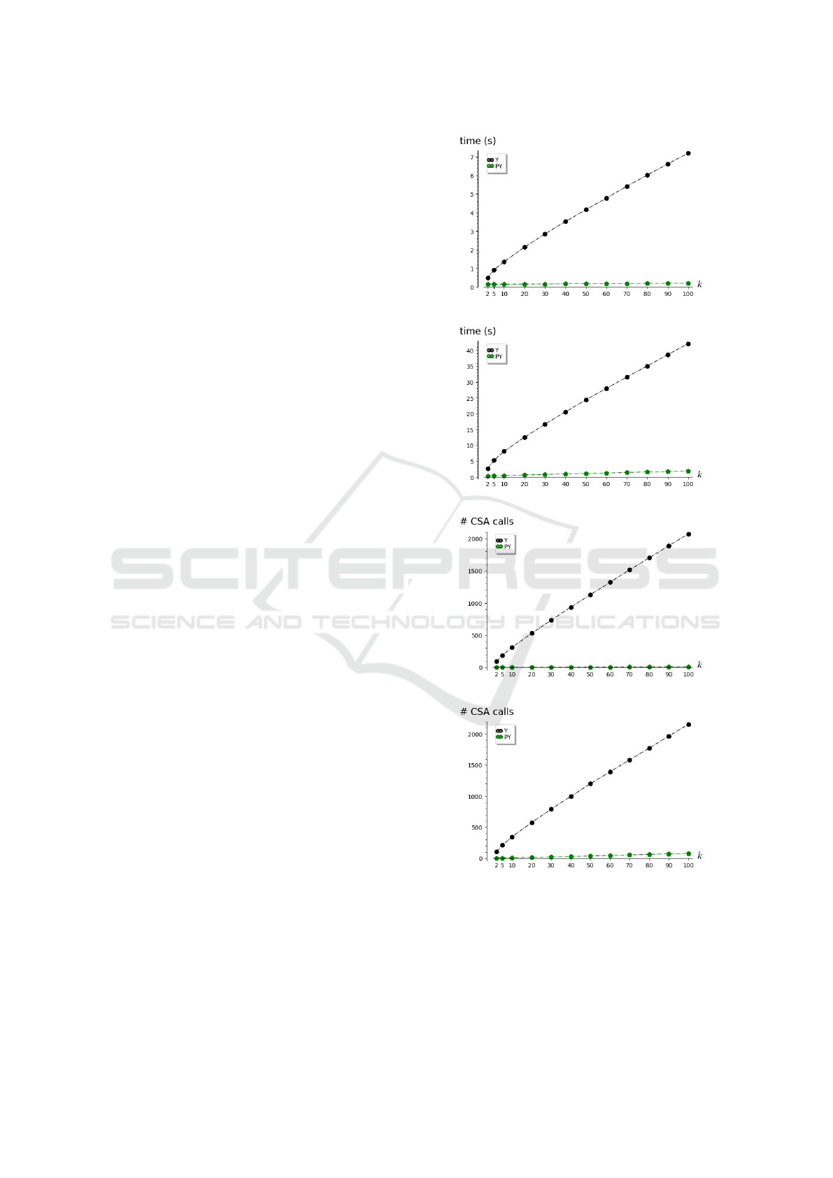
CSA calls) in Tables 2 and 3 and fig. 3 correspond to
the biggest experienced value of k (k = 100). While
the data in Figure 2 corresponds to their evolution
with respect to the values of k.
The average and median running times reported in
Table 2 show that the PY-PT algorithm is significantly
faster than the Y-PT algorithm for every considered
network (the average speed up of the running time is
bigger than a factor of 10 for k = 100). Moreover,
a refined comparison on the Germany and Paris net-
works (Figure 3) shows that PY-PT is faster than Y-PT
for almost all queries. In addition, Figures 2a and 2b
shows that this speed up remains considerable even
for small values of k (even for k = 2) for Stockholm
and Switzerland networks. This means that the time
consumed for the PCSA computation routine is com-
pensated by the extraction of simple detours, even for
k = 2. In addition, very similar results were obtained
on the remaining networks. Based on these remarks,
we conclude that, in practice, PY-PT is faster than Y-
PT for almost every scenario (the value of k, the query
specifications and the network structure).
Furthermore, on the Stockholm and Switzerland
networks, Table 3 and figs. 2c and 2d show that the
number of CSA calls is significantly reduced using
PY-PT. This ensures that a similar speed up is guar-
anteed for any experimental settings (Johnson, 2002).
As the obtained results are similar, we only dis-
played data obtained from experiments on selected
networks (Stockolm and Switzerland for Figure 2,
Paris and Germany for Figure 3). However, the re-
sults/plots corresponding to the remaining networks
are very similar.
To conclude, on average, PY-PT algorithm is more
than 10 times faster than Y-PT algorithm, it is also
faster than Y-PT for almost every scenario.
7 (DIS)SIMILARITY OF THE
OUTPUT JOURNEYS
In this section, we experimentally evaluate the dissim-
ilarity of the journeys extracted by our algorithms on
the described dataset in order to check whether our
algorithms can be used to extract dissimilar journeys.
Roughly, two journeys are similar if they share a
major part of their connections and footpaths. Here,
(a) Average running time on Stockholm.
(b) Average running time on Switzerland.
(c) Average number of CSA calls on Stockholm.
(d) Average number of CSA calls on Switzerland.
Figure 2: The running time of the kEAT algorithms on
Switzerland train network and Stockholm public transit net-
work with respect to the values of k.
analogously with the Jaccard similarity measure of
paths in graphs, that measures the similarity of two
paths by the ratio of the length of the arcs they have in
common over the length of their union (eq. 1) (Chon-
On Finding k Earliest Arrival Time Journeys in Public Transit Networks
323
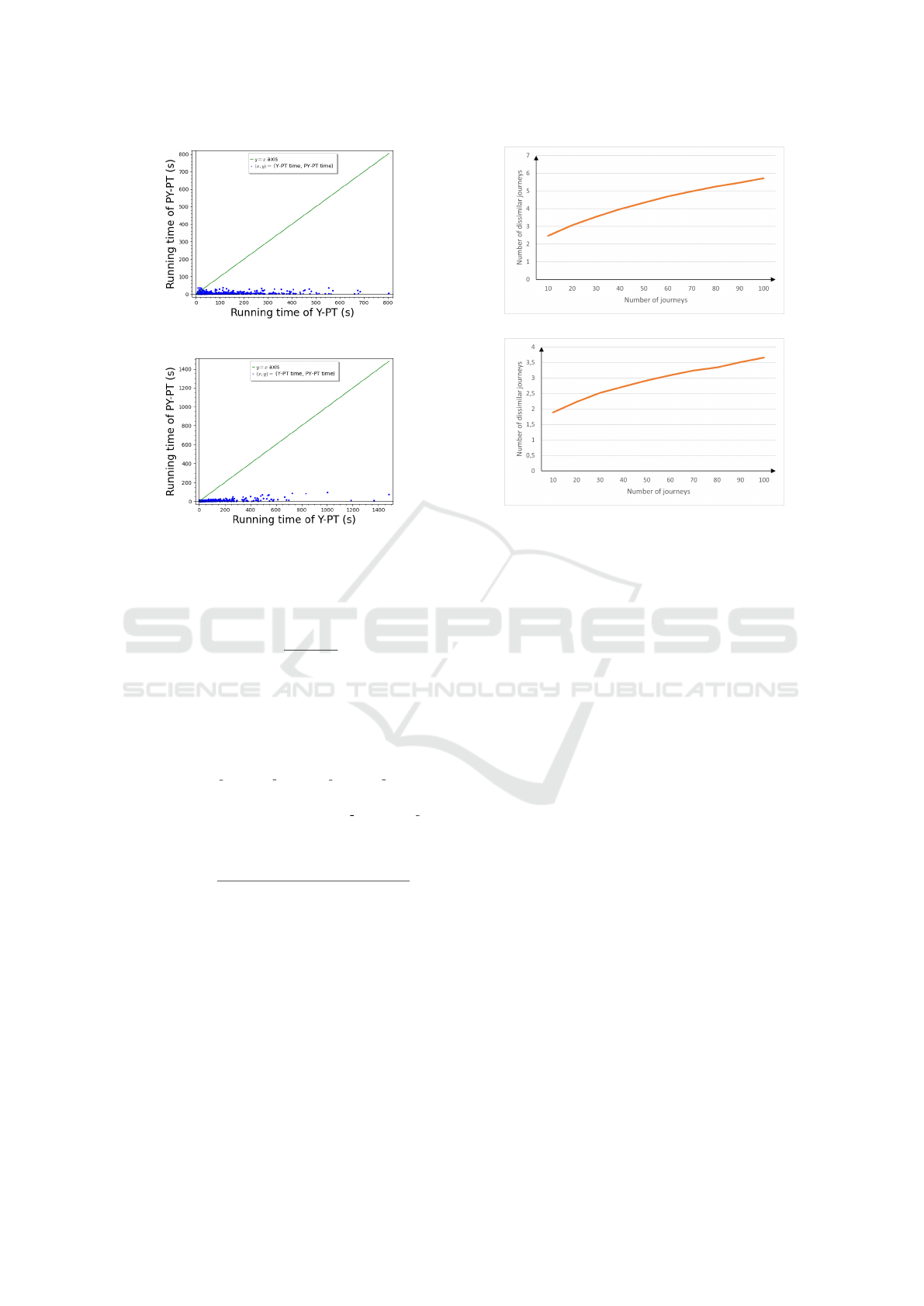
(a) Running time of Y-PT and PY-PT on Germany.
(b) Running time of Y-PT and PY-PT on Paris.
Figure 3: Comparison of the running time of Y-PT and PY-
PT on a train network and a public transit network.
drogiannis et al., 2017; Al Zoobi et al., 2021b).
S(P,Q) =
ℓ(P ∩Q)
ℓ(P ∪Q)
(1)
We define the similarity of two journeys as the ra-
tio between the travel time of their connections and
footpaths in common over the travel time of the union
of their connections and footpaths. Precisely, we de-
fine the similarity of two journeys as follows.
Let c = (c
dep stop
,c
arr stop
,c
dep time
,c
arr time
,c
trip
)
be a connection, we define the travel time of c as the
time consumed by c, i.e, dur(c) = c
arr time
−c
dep time
.
Now, let J
1
,J
2
be two journeys, the similarity between
J
1
and J
2
can be measured as follows.
S
PT
(J
1
,J
2
) =
∑
c∈J
1
∩J
2
dur(c)+
∑
f ∈J
1
∩J
2
f
dur
∑
c∈J
1
∪J
2
dur(c)+
∑
f ∈J
1
∪J
2
f
dur
(2)
So, given a threshold value θ ∈ [0,1], two journeys
J
1
and J
2
are called θ dissimilar if their similarity does
not exceed θ, i.e., if S
PT
(J
1
,J
2
) ≤ θ.
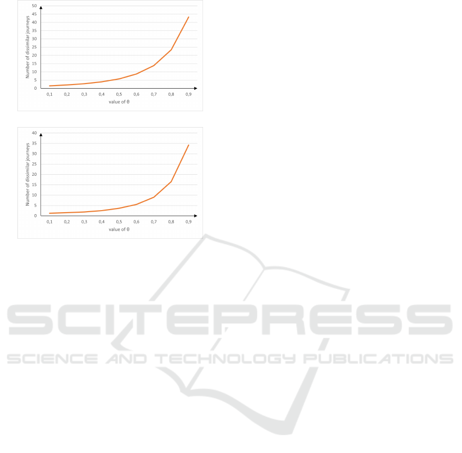
In order to evaluate the number of dissimilar jour-
neys given by our algorithms, we measured the num-
ber of journeys that are θ dissimilar among the first
100 journeys given by our algorithm. As shown in
Figure 4, our algorithms can be used to extract, on av-
erage, 3 to 5 journeys that are 0.5 dissimilar for the
Paris network. Moreover, Figure 5 shows the num-
ber of dissimilar journeys among the 100 journeys
given by our algorithms with respect to the value of
(a) Paris
(b) Germany
Figure 4: Number of paths that are 0.5 dissimilar among
those given by our algorithms.
the similarity measure θ. We notice that, starting from
θ = 0.8, the number of dissimilar journeys starts to be
considerable (more than 15 journeys).
The plots presented in this section corresponds to
the results obtained on the Paris and Germany net-
works. However, very similar results were obtained
on the remaining networks.
Summarizing, after measuring the similarity of the
journeys given by our algorithms in practice, we claim
that algorithms Y-PT and PY-PT can be used as a tool
to extract journeys that are reasonably dissimilar.
8 CONCLUSION
In this paper, we have explored alternative journey
planning in public transit networks, offering a vast
set of interesting solutions. This is done by adapting
the k shortest simple paths problem to the public tran-
sit network context. We proposed a straightforward
adaptation of Yen’s algorithm and a more refined ver-
sion answering the proposed problem in a reasonable
running time. Finally, we evaluated the similarity of
the output journeys and showed that our algorithms
can be used to extract dissimilar journeys.
Interesting questions are asked about designing al-
gorithms answering k earliest arrival journeys query
faster. Whether by improving / proposing faster meth-
ods than PY-PT algorithm, or even with the help of a
preprocessing routine. For instance, a more specific
ICORES 2022 - 11th International Conference on Operations Research and Enterprise Systems
324
(a) Paris
(b) Germany
Figure 5: Number of dissimilar paths among the first 100
paths given by our algorithms with respect to the variation
of the similarity threshold θ.
question is whether one can use journey planning al-
gorithms like Transfer Patterns algorithm (Bast et al.,
2010) to answer k earliest arrival journeys queries.
Another interesting question concerns the design
of algorithms dedicated to extracting dissimilar jour-
neys in public transit networks. This could be done
by adapting some of the algorithms proposed to find
shortest dissimilar paths in a graph (Chondrogiannis
et al., 2017).
REFERENCES
Al Zoobi, A., Coudert, D., and Nisse, N. (2020). Space
and time trade-off for the k shortest simple paths prob-
lem. In 18th International Symposium on Experimen-
tal Algorithms (SEA), volume 160, page 13. Schloss
Dagstuhl–Leibniz-Zentrum f
¨
ur Informatik.
Al Zoobi, A., Coudert, D., and Nisse, N. (2021a). Finding
the k Shortest Simple Paths: Time and Space trade-
offs. Research Report hal-03196830, Inria ; I3S, Uni-
versit
´
e C
ˆ
ote d’Azur.
Al Zoobi, A., Coudert, D., and Nisse, N. (2021b). On the
complexity of finding k shortest dissimilar paths in a
graph. Research Report hal-03187276, Inria ; CNRS
; I3S ; UCA.
Al Zoobi, A. and Finkelstein, A. (2021). PT-KSSP Github
Project. https://github.com/fink-arthur/PT-KSSP.
Barrett, C., Bisset, K., Holzer, M., Konjevod, G., Marathe,
M., and Wagner, D. (2008). Engineering label-
constrained shortest-path algorithms. In International
conference on algorithmic applications in manage-
ment, pages 27–37. Springer.
Bast, H., Carlsson, E., Eigenwillig, A., Geisberger, R., Har-
relson, C., Raychev, V., and Viger, F. (2010). Fast
routing in very large public transportation networks
using transfer patterns. In 18th Annual European Sym-
posium on Algorithms (ESA), pages 290–301.
Bast, H., Delling, D., Goldberg, A., M
¨
uller-Hannemann,
M., Pajor, T., Sanders, P., Wagner, D., and Wer-
neck, R. F. (2016). Route planning in transportation
networks. In Algorithm engineering, pages 19–80.
Springer.
Chondrogiannis, T., Bouros, P., Gamper, J., and Leser, U.
(2017). Exact and approximate algorithms for finding
k-shortest paths with limited overlap. In 20th Interna-
tional Conference on Extending Database Technology
(EDBT), pages 414–425.
Delling, D., Pajor, T., and Werneck, R. F. (2015). Round-
based public transit routing. Transportation Science,
49(3):591–604.
Dibbelt, J., Pajor, T., Strasser, B., and Wagner, D. (2018).
Connection scan algorithm. ACM Journal of Experi-
mental Algorithmics (JEA), 23:1–56.
Eppstein, D. (1998). Finding the k shortest paths. SIAM
Journal on Computing, 28(2):652–673.
Johnson, D. S. (2002). A theoretician’s guide to the exper-
imental analysis of algorithms. Data structures, near
neighbor searches, and methodology: fifth and sixth
DIMACS implementation challenges, 59:215–250.
Kurz, D. and Mutzel, P. (2016). A sidetrack-based al-
gorithm for finding the k shortest simple paths in
a directed graph. In 27th International Symposium
on Algorithms and Computation (ISAAC), volume 64
of LIPIcs, pages 49:1–49:13. Schloss Dagstuhl -
Leibniz-Zentrum f
¨
ur Informatik.
Scano, G., Huguet, M.-J., and Ngueveu, S. U. (2015).
Adaptations of k-shortest path algorithms for trans-
portation networks. In International Conference
on Industrial Engineering and Systems Management
(IESM), pages 663–669. IEEE.
Schulz, F., Wagner, D., and Weihe, K. (2000). Dijkstra’s
algorithm on-line: An empirical case study from pub-
lic railroad transport. ACM Journal of Experimental
Algorithmics (JEA), 5:12–es.
Vo, K. D., Pham, T. V., Nguyen, H. T., Nguyen, N., and
Van Hoai, T. (2015). Finding alternative paths in city
bus networks. In 2015 International Conference on
Computer, Control, Informatics and its Applications
(IC3INA), pages 34–39. IEEE.
Yen, J. Y. (1971). Finding the k shortest loopless paths in a
network. Management Science, 17(11):712–716.
On Finding k Earliest Arrival Time Journeys in Public Transit Networks
325
